From Entropy to KL Divergence: A Comprehensive Guide
KL Divergence, one of the most important concepts in information theory and statistics, measures the difference between two probability distributions. It quantifies how much information is lost when one distribution is used to approximate another. It is widely used in various fields, including machine learning, data science, and artificial intelligence. In this blog post, we will explore the concept of KL Divergence, its mathematical formulation, and its applications.
First, let’s start with the concept of entropy, which is the foundation of KL Divergence.
1 Entropy
Entropy is a measure of uncertainty or randomness in a probability distribution. It quantifies the average amount of information required to describe the outcome of a random variable.
First, let’s define what is the information content of an event. Intuitively, the information should have the following two properties:
- The less likely an event is to occur, the more information it provides when it does occur. Mathematically, this means that the information content should be inversely proportional to the probability of the event.
- The information content of independent events should be additive. This means that if two events are independent, the total information content should be the sum of the individual information contents.
Based on these properties, we can define the information content \(I(x)\) of an event \(x\) with probability \(P(x)\) as:
\[ I(x) = -\log P(x) \tag{1}\]
The negative logarithm ensures that the information content is non-negative and satisfies the two properties mentioned above. One small note is that the base of the logarithm determines the unit of information. For example, if we use base 2, the unit is bits; if we use base \(e\), the unit is nats. In the deep learning community, we often use nats as the unit of information.
Ok, we have define the information content of an event. Now, we can define the entropy of a probability distribution, which is the average information content of all possible events in the distribution. When we say “average”, we mean the expectation over the distribution, so the entropy can be defined as:
\[ H(P) = \mathbb{E}_{x \sim P} [I(x)] = \mathbb{E}_{x \sim P} [-\log P(x)] \tag{2}\]
For the discrete case, the entropy is defined as:
\[ H(P) = -\sum_{x} P(x) \log P(x) \tag{3}\]
where the sum is taken over all possible outcomes \(x\) of the random variable.
For the continuous case, the entropy is defined as: \[ H(P) = -\int P(x) \log P(x) dx \tag{4}\]
where the integral is taken over the entire support of the random variable. The entropy for continuous distributions is also known as differential entropy.
NOTE: Entropy in Physics
The content of entropy was originally introduced as a thermodynamic quantity that measures the number of microscopic configurations (microstates) corresponding to a macroscopic state (macrostate).
In physics, entropy is a quantitative measure of uncertainty over microscopic states, given limited macroscopic information.
A physical system can be described at two levels:
- Macroscopic state: observable quantities (temperature, pressure, energy)
- Microscopic state: the exact configuration of all particles
Many different microscopic configurations can correspond to the same macroscopic observation. Entropy measures how many possibilities remain unresolved.
In statistical mechanics, this idea is captured by Boltzmann entropy: \[ S = k_B \log \Omega \] where \(\Omega\) is the number of microscopic states consistent with the observed constraints.
This concept directly generalizes to probability distributions. When microstates are not equally likely, uncertainty is no longer determined by counting, but by averaging surprisal: \[ H(P) = -\sum_x P(x)\log P(x) \]
From a modern perspective: - Thermodynamic entropy quantifies uncertainty over physical configurations - Shannon entropy quantifies uncertainty over random variables - Both arise from the same principle: maximum uncertainty subject to constraints
This principle is fundamental in machine learning: - Maximum entropy leads to exponential-family distributions - Many learning objectives can be derived from entropy maximization or entropy regularization - KL divergence, cross-entropy, and likelihood-based training all build on this foundation
Thus, entropy provides a unifying abstraction that links physics, information theory, and modern deep learning objectives.
1.1 Maximum Entropy Principle
The maximum entropy principle states that, given a set of constraints, the probability distribution that best represents the current state of knowledge is the one with the maximum entropy. This principle is often used in statistical mechanics and machine learning to derive probability distributions that satisfy certain constraints while making the least amount of assumptions about the data.
We can formulate the maximum entropy problem as follows: Given a set of constraints on the expected values of certain functions \(f_i(x)\), we want to find the probability distribution \(P(x)\) that maximizes the entropy subject to these constraints:
\[ \begin{split} \text{maximize} \quad & H(P) = -\sum_{x} P(x) \log P(x) \\ \text{subject to} \quad & \sum_{x} P(x) f_i(x) = c_i, \quad i = 1, 2, \ldots, m \\ & \sum_{x} P(x) = 1 \\ & P(x) \geq 0, \quad \forall x \end{split} \tag{5}\]
where \(c_i\) are the expected values of the functions \(f_i(x)\). The solution to this optimization problem can be found using the method of Lagrange multipliers, leading to the following form for the maximum entropy distribution: \[ P(x) = \frac{1}{Z} \exp\left(-\sum_{i=1}^{m} \lambda_i f_i(x)\right) \tag{6}\]
where \(\lambda_i\) are the Lagrange multipliers and \(Z\) is the partition function that normalizes the distribution. Solving for the Lagrange multipliers \(\lambda_i\) allows us to find the maximum entropy distribution that satisfies the given constraints. The solution for \(\lambda_i\) typically requires numerical methods, as it involves solving a system of equations derived from the constraints. Solve these equations to obtain the specific values of \(\lambda_i\) that define the maximum entropy distribution. For the diescrete case, the partition function \(Z\) is given by: \[ Z = \sum_{x} \exp\left(-\sum_{i=1}^{m} \lambda_i f_i(x)\right) \tag{7}\]
For the continuous case, the partition function \(Z\) is given by: \[ Z = \int \exp\left(-\sum_{i=1}^{m} \lambda_i f_i(x)\right) dx \tag{8}\]
Solve the above, we can obtain the maximum entropy distribution that satisfies the given constraints:
For the discrete case: \[ P(x) = \frac{1}{\sum_{x} \exp\left(-\sum_{i=1}^{m} \lambda_i f_i(x)\right)} \exp\left(-\sum_{i=1}^{m} \lambda_i f_i(x)\right) \tag{9}\]
For the continuous case: \[ P(x) = \frac{1}{\int \exp\left(-\sum_{i=1}^{m} \lambda_i f_i(x)\right) dx} \exp\left(-\sum_{i=1}^{m} \lambda_i f_i(x)\right) \]
1.2 Applications of Entropy
Entropy and Maximum Entropy Principle have wide-ranging applications in various fields, for example: - Data Compression: Entropy is used to determine the optimal encoding scheme for data compression. The lower the entropy, the more compressible the data is. - Cryptography: Entropy is used to measure the randomness of cryptographic keys. Higher entropy keys are more secure against brute-force attacks. - Machine Learning: Entropy is used in decision tree algorithms to measure the impurity of a dataset. The goal is to minimize the entropy of the dataset after each split. - Information Theory: Entropy is a fundamental concept in information theory, where it is used to quantify the amount of information in a message.
TL;DR: Entropy
Entropy is a measure of uncertainty in a probability distribution. It quantifies the average amount of information required to describe the outcome of a random variable. The categorical formula for entropy is uniforma distribution, for the continuous case, the entropy of a standard normal distribution is approximately 1.418 nats.
For example, in the reinforcement learning, entropy regularization is often used to encourage exploration by adding an entropy term to the reward function. This helps to prevent the agent from getting stuck in local optima and promotes more diverse behavior.
2 Cross-Entropy
Cross-entropy measures the difference between two probability distributions. It quantifies the average number of bits needed to identify an event from a set of possibilities, given a predicted probability distribution \(Q\) instead of the true distribution \(P\). The cross-entropy \(H(P, Q)\) is defined as: \[ H(P, Q) = -\sum_{x} P(x) \log Q(x) \tag{10}\]
For the continuous case, the cross-entropy is defined as: \[ H(P, Q) = -\int P(x) \log Q(x) dx \tag{11}\]
Look very similar to entropy (Equation 3), right? The only difference is that in cross-entropy, we use the predicted distribution \(Q\) instead of the true distribution \(P\) in the logarithm term.
3 KL Divergence
After understanding entropy and cross-entropy, we can now define KL Divergence.
KL Divergence measures the difference between two probability distributions \(P\) and \(Q\). It quantifies the amount of information lost when \(Q\) is used to approximate \(P\). The KL Divergence \(D_{KL}(P || Q)\) is defined as: \[ D_{KL}(P || Q) = \mathbb{E}_{x \sim P} \left[ \log \frac{P(x)}{Q(x)} \right] \tag{12}\]
For the discrete case, the KL Divergence is defined as: \[ D_{KL}(P || Q) = \sum_{x} P(x) \log \frac{P(x)}{Q(x)} \tag{13}\]
For the continuous case, the KL Divergence is defined as:
\[ D_{KL}(P || Q) = \int P(x) \log \frac{P(x)}{Q(x)} dx \tag{14}\]
Let’s expand the definition of KL Divergence to see its relationship with entropy(Equation 2) and cross-entropy(Equation 10):
\[ \begin{split} D_{KL}(P || Q) & = \mathbb{E}_{x \sim P} \left[ \log \frac{P(x)}{Q(x)} \right] \\ & = - \underbrace{\mathbb{E}_{x \sim P}[-\log P(x)]}_{\text{Entropy } H(P)} + \underbrace{\mathbb{E}_{x \sim P}[-\log Q(x)]}_{\text{Cross-Entropy } H(P, Q)} \\ & = H(P, Q) - H(P) \end{split} \tag{15}\]
We can see from Equation 15, KL Divergence can be interpreted as the difference between cross-entropy and entropy. In other words, it measures how much more information is needed to encode samples from distribution \(P\) using the code optimized for distribution \(Q\) instead of the optimal code for \(P\).
def kl_divergence(p: torch.Tensor, q: torch.Tensor):
    return torch.sum(p * torch.log((p + 1e-10) / (q + 1e-10)))
KL Divergence has several important properties, each of which has significant implications in various applications:
- Asymmetry: KL Divergence is not symmetric, meaning that \(D_{KL}(P || Q) \neq D_{KL}(Q || P)\). This property reflects the fact that KL Divergence measures the information lost when approximating \(P\) with \(Q\), and not vice versa.
- Non-negativity: KL Divergence is always non-negative, i.e., \(D_{KL}(P || Q) \geq 0\), with equality if and only if \(P = Q\) almost everywhere. This property is a consequence of Gibbs’ inequality.
- Additivity: KL Divergence is additive for independent distributions. If \(P_1\) and \(P_2\) are independent distributions, and \(Q_1\) and \(Q_2\) are independent distributions, then: \[ D_{KL}(P_1 \times P_2 || Q_1 \times Q_2) = D_{KL}(P_1 || Q_1) + D_{KL}(P_2 || Q_2) \]
- Invariance under parameterization: KL Divergence is invariant under reparameterization of the distributions. If \(f\) is a bijective function, then: \[ D_{KL}(P || Q) = D_{KL}(f(P) || f(Q)) \]
Let’s take a closer look at some of these properties.
3.1 KL Divergence Properties
In the previous section, we have seen the defination of the KL-Divergence, and the relation between KL-Divergence, entropy and cross entropy. In this section, let’s see some properties of the KL divergence.
3.1.1 Asymmetry of KL Divergence
The first property of KL Divergence is that it is asymmetric, meaning that \(D_{KL}(P || Q) \neq D_{KL}(Q || P)\). This asymmetry reflects the fact that KL Divergence measures the information lost when approximating \(P\) with \(Q\), and not vice versa.
Here we assume that \(P\) is the true distribution, and \(Q\) is the model distribution that we are using to approximate \(P\).
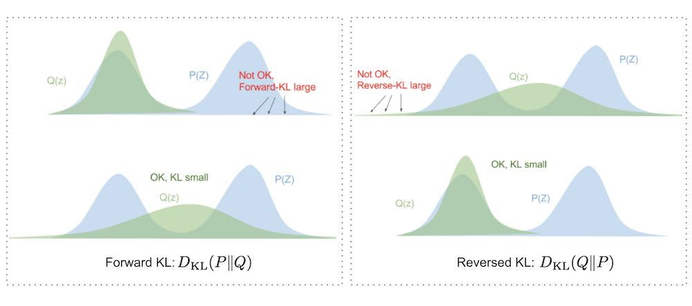
So, \(D_{KL}(P || Q)\) is known as the forward KL Divergence, while \(D_{KL}(Q || P)\) is known as the reverse KL Divergence. The choice between using forward or reverse KL Divergence depends on the specific application and the properties of the distributions involved. We will dig deeper into this topic in the applications section (Section 5.5) later.
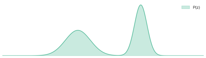
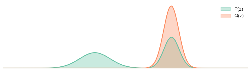
Let’s see how this asymmetry property affects the optimization of model parameters in practice through a toy example: \(P = \sum_{i=1}^2 \frac{1}{2} \mathcal{N}(\mu_i, \sigma_i)\), where \(\mu_1 = -2\) and \(\mu_2 = 3\). We want to use a single Gaussian distribution \(Q_{\theta} = \mathcal{N}(\mu, \sigma^2)\) to approximate the true distribution \(P\). We will optimize the model parameters \(\theta = (\mu, \sigma)\) using both forward and reverse KL Divergence.
import torch.distributions as D
P = D.MixtureSameFamily(
    D.Categorical(torch.tensor([0.5, 0.5])),
    D.Normal(
        loc=torch.tensor([-2.0, 3.0]),
        scale=torch.tensor([1.0, 0.5]),
    ),
)
3.1.1.1 Forward KL Divergence
For the forward KL Divergence, we need to solve:
\[ \begin{split} D_{KL}(P || Q_{\theta}) & = \mathbb{E}_{x \sim P} \left[ \log \frac{P(x)}{Q_{\theta}(x)} \right] \\ & = \mathbb{E}_{x \sim P} [\log P(x)] - \mathbb{E}_{x \sim P} [\log Q_{\theta}(x)] \\ & =\boxed{- \mathbb{E}_{x \sim P} [\log Q_{\theta}(x)] } + \text{constant} \end{split} \tag{16}\]
As we can see from Equation 16, when we minimize the forward KL Divergence, we are essentially maximizing the expected log-likelihood of the model distribution \(Q_{\theta}\) under the true distribution \(P\)..
So, the forward KL Divergence is equivalent to the maximum likelihood estimation (MLE) objective:
\[ \begin{split} \mathcal{L}_{\text{MLE}} &= - \mathbb{E}_{x \sim P} [\log Q_{\theta}(x)] \\ &\approx - \frac{1}{N} \sum_{i=1}^{N} \log Q_{\theta}(x_i) \end{split} \tag{17}\]
To optimize the model parameters \(\theta\), we need to have:
- Samples \(x \sim P\) from the true distribution \(P\) or the true data distribution \(P\).
- The ability to compute the log-likelihood of the model distribution \(Q_{\theta}\) for those samples.
So, to minimize the forward KL Divergence, we just need to maximize the likelihood of the model distribution \(Q_{\theta}\) on the data samples drawn from the true distribution \(P\).
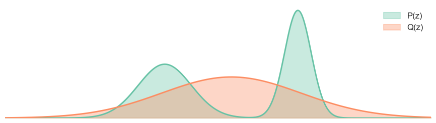
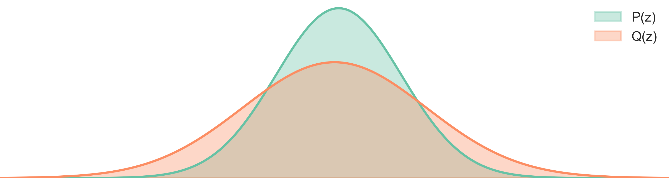
As we can see from the figure above, when we minimize the forward KL Divergence, the model distribution \(Q_{\theta}\) will try to cover all the modes of the true distribution \(P\), even if it means putting some probability mass on low-likelihood regions. This is because the forward KL Divergence penalizes missing modes more heavily than putting mass on low-likelihood regions.
3.1.1.2 Backward KL Divergence
For the reverse KL Divergence, we need to solve:
\[ \begin{split} D_{KL}(Q_{\theta} || P) & = \mathbb{E}_{x \sim Q_{\theta}} \left[ \log \frac{Q_{\theta}(x)}{P(x)} \right] \\ & = \mathbb{E}_{x \sim Q_{\theta}} [\log Q_{\theta}(x)] - \mathbb{E}_{x \sim Q_{\theta}} [\log P(x)] \\ & = \mathbb{E}_{x \sim Q_{\theta}} [- \log P(x)] - \mathbb{E}_{x \sim Q_{\theta}} [- \log Q_{\theta}(x)] \\ & = H(Q_{\theta}, P) - H(Q_{\theta}) \\ \end{split} \tag{18}\]
As we can see from Equation 18, when we minimize the reverse KL Divergence, we are essentially minimizing the expected negative log-likelihood of the true distribution \(P\) under the model distribution \(Q_{\theta}\). We need:
- Samples \(x \sim Q_{\theta}\) from the model distribution \(Q_{\theta}\).
- The ability to compute the log-likelihood of the true distribution \(P\) for those samples.
So, to minimize the reverse KL Divergence, means: choose the model parameters \(\theta\) such that the model distribution \(Q_{\theta}\) generates samples that have high likelihood under the true distribution \(P\)(lower cross entropy) while avoid putting too much probability mass on low-likelihood regions (higher entropy).
In sentence:
Minimizing reverse KL means: “Make Q put its mass only where P is high; it’s okay if Q misses parts of P.”
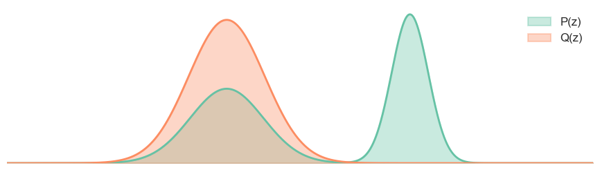
NOTE: About the iniltiazation
One thing to note that, since we use gradient descent to get the optimal \(\theta\), the initalization matters. In the Figure 4, we initalize the $= -2 $, but if we initalize the \(\mu = 3\), the result will be different:
Let’s summarize the difference between forward and reverse KL Divergence:
| Aspect | Equation | Equalent Objective | Requirements | Behavior |
|---|---|---|---|---|
| Forward KL Divergence | \(D_{KL}(P || Q_{\theta}) = \mathbb{E}_{x \sim P} \left[ \log \frac{P(x)}{Q_{\theta}(x)} \right]\) | max \(- \mathbb{E}_{x \sim P} [\log Q_{\theta}(x)]\) | 1. Samples from \(P\) or Sampable \(P\) , 2.ability to compute \(\log Q_{\theta}(x)\) | Covers all modes of \(P\), even if it means putting mass on low-likelihood regions |
| Reverse KL Divergence | \(D_{KL}(Q_{\theta} || P) = \mathbb{E}_{x \sim Q_{\theta}} \left[ \log \frac{Q_{\theta}(x)}{P(x)} \right]\) | Minimize expected negative log-likelihood of \(P\) under \(Q_{\theta}\) | Samples from \(Q_{\theta}\), ability to compute \(\log P(x)\) | Focuses on high-likelihood regions of \(P\), may miss some modes |
Different applications may require different choices between forward and reverse KL Divergence, depending on the specific goals and properties of the distributions involved. For example, in the classification task, we often use forward KL Divergence (Equation 16) to train the model, while in the generative modeling task, we often use reverse KL Divergence (Equation 18) to train the model. We will discuss these applications in more details later (Section 5.1, Section 5.2).
3.1.2 Non-Negativity of KL Divergence
Another important property of KL Divergence is that it is always non-negative, i.e., \(D_{KL}(P || Q) \geq 0\), with equality if and only if \(P = Q\) almost everywhere. This property is a consequence of Gibbs’ inequality. We can prove this using Jensen’s inequality: \[ D_{KL}(P || Q) = \mathbb{E}_{x \sim P} \left[ -\log \frac{Q(x)}{P(x)} \right] \geq -\log \mathbb{E}_{x \sim P} \left[ \frac{Q(x)}{P(x)} \right] = \log 1 = 0 \]
Because the logarithm function is concave, we can apply Jensen’s inequality to obtain the above result. The equality holds if and only if \(P(x) = Q(x)\) for all \(x\) in the support of \(P\).
This property is important because it ensures that KL Divergence is a valid measure of the difference between two probability distributions. If KL Divergence could be negative, it would not make sense as a measure of divergence.
We will see the implications of this property in various applications of KL Divergence later (Section 5.2).
3.1.3 Additivity of KL Divergence
KL Divergence is additive for independent distributions. If \(P_1\) and \(P_2\) are independent distributions, and \(Q_1\) and \(Q_2\) are independent distributions, then:
\[ D_{KL}(P_1 \times P_2 || Q_1 \times Q_2) = D_{KL}(P_1 || Q_1) + D_{KL}(P_2 || Q_2) \tag{19}\]
This property is useful when we want to compute the KL Divergence between two joint distributions that factorize into independent components. It allows us to compute the KL Divergence for each component separately and then sum them up to get the total KL Divergence. This can significantly reduce the computational complexity when dealing with high-dimensional distributions that factorize into independent components. (Though in practice, many distributions do not factorize into independent components, so this property may not always be applicable.)
3.1.4 Invariance under Reparameterization
KL Divergence is invariant under reparameterization of the distributions. If \(f\) is a bijective function, then:
\[ D_{KL}(P || Q) = D_{KL}(f(P) || f(Q)) \tag{20}\]
This property means that the KL Divergence between two distributions is not affected by how we parameterize those distributions. For example, if we have two Gaussian distributions \(P\) and \(Q\), and we reparameterize them using a bijective function (e.g., a linear transformation), the KL Divergence between the reparameterized distributions will be the same as the KL Divergence between the original distributions. This property is important because it allows us to choose different parameterizations for our models without affecting the KL Divergence, which can be useful for optimization and numerical stability.
3.2 Monte Carlo Estimation
Knowing what is the KL Divergence and its properties, the next question is: how to estimate KL Divergence in practice? In the reality, we sometimes don’t have true distribution \(P\), what we have is \(\mathcal{D} = \{x_1, x_2, \ldots, x_N\}\), a set of samples drawn from distribution \(P\). But we want is use \(Q\) to approximate \(P\), and we want to measure how good is the approximation using KL Divergence. Ok, what can we do? Well, we can use Monte Carlo estimation to estimate the KL Divergence using the samples from distribution \(P\). Why we need Monte Carlo estimation? We need MC estimation because:
- The distribution \(P\) or \(Q\) may not have a closed-form expression, making it difficult to compute the KL Divergence analytically.
- The dimensionality of the data may be high, making numerical integration methods computationally expensive
- We may only have access to samples from the distribution \(P\), rather than the full distribution itself.
In this section, we will explore the first two cases, where we have access to the full distribution \(P\) and \(Q\), but they may not have closed-form expressions or may be high-dimensional. For the third case, where we only have access to samples from distribution \(P\), we will discuss it in the next section (Section 5.2).
We will derive three Monte Carlo estimation methods for KL Divergence:
- Naive Monte Carlo Estimation
- Importance Sampling
- Control Variates
3.2.1 Naive Monte Carlo Estimation
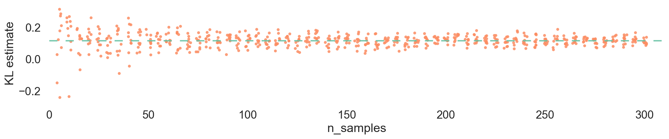
The Monte Carlo estimation of KL Divergence involves using samples drawn from distribution \(P\) to estimate the expectation in the definition of KL Divergence. Given a set of samples \(\{x_1, x_2, \ldots, x_N\}\) drawn from distribution \(P\), we can estimate the KL Divergence as follows:
\[ D_{KL}(P || Q) \approx \frac{1}{N} \sum_{i=1}^{N} \log \frac{P(x_i)}{Q(x_i)} \tag{21}\]
This is un-biased estimator of KL Divergence using samples from distribution \(P\). However, it may have high variance depending on the number of samples and the distributions involved.
3.2.2 Variance Reduction
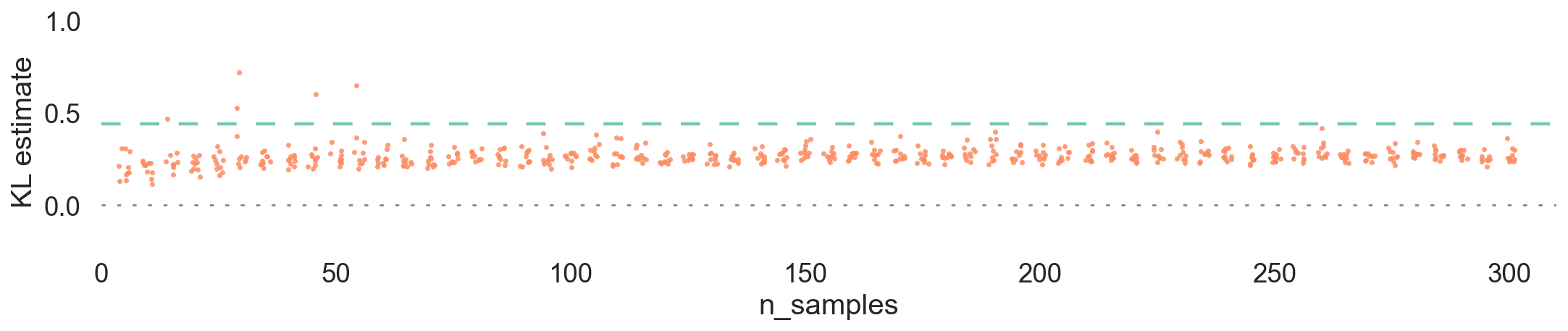
WAIT! we just mentioned that KL divergence is non-negative, but in the above figure, we can see that the estimated KL Divergence is negative when using 10 samples. Why is that? The problem arise in the \(\log\) term, when \(Q(x_i)\) is bigger than \(P(x_i)\), the \(\log\) term becomes negative, and when we average over all samples, the estimated KL Divergence can become negative. This is a limitation of the naive Monte Carlo estimation method, especially when the number of samples is small or when the distributions \(P\) and \(Q\) are very different.
One way to address this issue is to write the KL Divergence as:
\[ \widehat{D_{KL}}(P || Q) = \frac{1}{N} \sum_{i=1}^{N} \frac{1}{2} \left( \log \frac{P(x_i)}{Q(x_i)} \right)^2 \tag{22}\]
NOTE Derive of Equation 22
For those interested in the derivation of Equation 22, here it is. Let’s define a new random variable \(r\) as: \(r=\frac{Q}{P}\). Then, we can rewrite the KL Divergence as:
\[ D_{KL}(P || Q) = \mathbb{E}_{x \sim P} \left[ -\log r(x) \right] \]
Now, we can use the Taylor expansion of the logarithm function around \(r=1\) (i.e., when \(P \approx Q\)): \[ -\log r \approx (1 - r) + \frac{(1 - r)^2}{2} + O((1 - r)^3) \]
Taking the expectation with respect to \(P\), we have: \[ D_{KL}(P || Q) \approx \mathbb{E}_{x \sim P} \left[ (1 - r(x)) + \frac{(1 - r(x))^2}{2} \right] \]
Since \(\mathbb{E}_{x \sim P}[1 - r(x)] = 0\), the first term vanishes, and we are left with: \[ D_{KL}(P || Q) \approx \frac{1}{2} \mathbb{E}_{x \sim P} \left[ (1 - r(x))^2 \right] \] Expanding \((1 - r(x))^2\), we get: \[ (1 - r(x))^2 = \left(1 - \frac{Q(x)}{P(x)}\right)^2 = \left(\frac{P(x) - Q(x)}{P(x)}\right)^2 = \left(\frac{P(x)}{Q(x)} - 1\right)^2 \]
Substituting this back into the expectation, we have: \[ D_{KL}(P || Q) \approx \frac{1}{2} \mathbb{E}_{x \sim P} \left[ \left(\frac{P(x)}{Q(x)} - 1\right)^2 \right] \]
In the begin, we assume that \(P \approx Q\), which means that \(\frac{P(x)}{Q(x)}\) is close to 1. Therefore, we have \(\left(\frac{P(x)}{Q(x)} - 1\right)^2 \approx \left(\log \frac{P(x)}{Q(x)}\right)^2\). Plugging this approximation into the expectation, we get:
\[ D_{KL}(P || Q) \approx \frac{1}{2} \mathbb{E}_{x \sim P} \left[ \left(\log \frac{P(x)}{Q(x)}\right)^2 \right] \]
We arrive at the estimator in Equation 22. Notice that we ignore the -1 term in the expansion, as it does not affect the estimation of KL Divergence.
Good, this is lower variance, but it is biased. So, is there any other way to reduce the variance while keeping the estimator unbiased?
3.2.3 Control Variates
We known the naive version Equation 21 is unbiased but high variance, while the second version Equation 22 is lower variance but biased. Is there any way to reduce the variance while keeping the estimator unbiased? Yes, we can use control variates to achieve this.
Control variates is a variance reduction technique that involves using a correlated variable with known expected value to reduce the variance of an estimator. In the context of KL Divergence estimation, we can use a control variate to improve the estimate:
\[ D_{KL}(P || Q) \approx \frac{1}{N} \sum_{i=1}^{N} \left( \log \frac{P(x_i)}{Q(x_i)} - \boxed{\lambda(g(x_i) - E[g(X)])} \right) \]
As long as the term \(\lambda(g(x_i) - E[g(X)])\) has zero mean under distribution \(P\), the estimator remains unbiased. Let’s first verify that the expectation of the control variate term is zero:
\[ \begin{split} \mathbb{E}_{x \sim P}[\lambda(g(x) - E[g(X)])] & = \lambda \left( \mathbb{E}_{x \sim P}[g(x)] - E[g(X)] \right) \\ & = \lambda (\int P(x) g(x) dx - E[g(X)]) \\ & = 0 \end{split} \]
where \(\lambda\) is a scaling factor that can be optimized to minimize the variance of the estimator, and \(g(x)\) is a function that is correlated with the log-ratio term \(\log \frac{P(x)}{Q(x)}\). The choice of \(g(x)\) is crucial for the effectiveness of the control variate method. A common choice for \(g(x)\) is to use a function that approximates the log-ratio term, such as a linear or quadratic function. Plug in the \(g(x)\) into the estimator, we have:
\[ D_{KL}(P || Q) \approx \frac{1}{N} \sum_{i=1}^{N} \left(- \log g(x_i) - \lambda\left(g(x_i) - 1 \right) \right) \tag{23}\]
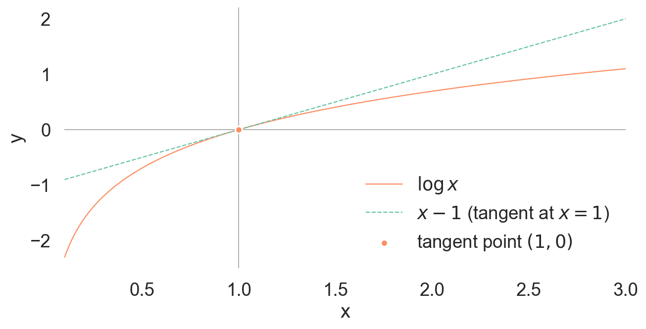
We see the \(x-1\) is always greater than or equal to 0 when \(x \geq 1\), and less than or equal to 0 when \(x \leq 1\). Therefore, by choosing an appropriate \(\lambda\), we can reduce the variance of the estimator.
We can take \(\lambda = 1\) for simplicity, and the estimator becomes: \[ D_{KL}(P || Q) \approx \frac{1}{N} \sum_{i=1}^{N} \left( g(x_i) - 1 - g(x_i) \right) \]
3.2.4 MC Estimation Summary
In this section, we have explored three Monte Carlo estimation methods for KL Divergence:
| Method | Form | Unbiased | Variance |
|---|---|---|---|
| Naive Monte Carlo | \(\frac{1}{N} \sum_{i=1}^{N} \log \frac{P(x_i)}{Q(x_i)}\) | Yes | High |
| Squared Log Estimator | \(\frac{1}{N} \sum_{i=1}^{N} \frac{1}{2}\left(\log \frac{P(x_i)}{Q(x_i)}\right)^2\) | No | Low |
| Control Variates | \(\frac{1}{N} \sum_{i=1}^{N}\!\left(\log \frac{P(x_i)}{Q(x_i)} - \lambda\big(g(x_i)-\mathbb{E}[g(X)]\big)\right)\) | Yes | Low |
4 \(f\)-Divergence
Before we dive into the applications of KL Divergence, let’s take a look at a more general class of divergence measures called \(f\)-Divergence. KL Divergence is actually a special case of \(f\)-Divergence.
\(f\)-Divergence is a class of divergence measures that quantify the difference between two probability distributions \(P\) and \(Q\). It is defined as:
\[ D_f(P || Q) = \mathbb{E}_{x \sim Q} \left[ f\left( \frac{P(x)}{Q(x)} \right) \right] \tag{24}\]
where \(f: (0, \infty) \to \mathbb{R}\) is a convex function satisfying \(f(1) = 0\). Different choices of the function \(f\) lead to different divergence measures. For example:
- KL Divergence: \(f(t) = t \log t\)
- Reverse KL Divergence: \(f(t) = -\log t\)
- Jensen-Shannon Divergence: \(f(t) = \frac{1}{2} \left( t \log t + (1 - t) \log (1 - t) \right)\)
- Total Variation Distance: \(f(t) = \frac{1}{2} |t - 1|\)
The \(f\)-Divergence framework provides a unified way to understand and analyze different divergence measures. The \(f\)-Divergence has several important properties, including non-negativity, convexity, and invariance under reparameterization. These properties make \(f\)-Divergence a useful tool in various applications, such as statistical inference, machine learning, and information theory.
5 Applications of KL Divergence
KL Divergence has numerous applications in various fields, including:
- Classification: KL Divergence is used as a loss function in classification tasks to measure the difference between the predicted probability distribution and the true distribution.
- Generative Models: KL Divergence is used in training generative models such as Variational Autoencoders (VAEs) to measure the difference between the learned distribution and the true data distribution.
- Model Distillation: KL Divergence is used to transfer knowledge from a large model (teacher) to a smaller model (student) by minimizing the KL Divergence between their output distributions.
- Reinforcement Learning: KL Divergence is used in policy optimization algorithms to ensure that the updated policy does not deviate too much from the previous policy.
- Large Language Models (LLMs): KL Divergence is used in post-training techniques such as Reinforcement Learning from Human Feedback (RLHF) to fine-tune LLMs to better align with human preferences
Do you still remember the asymmetry property (Section 3.1.1) of KL Divergence we discussed earlier ? This property plays a crucial role in many of these applications, as the choice between forward and reverse KL Divergence can significantly impact the behavior of the models being trained.
5.1 Supervised Regression and Classification
In the classification tasks, KL Divergence is often used as a loss function to measure the difference between the predicted probability distribution and the true distribution (one-hot encoded labels):
\[ \mathcal{L}_{\text{class}} = D_{KL}(P_{true} || P_{pred}) = \sum_{j}^N \sum_{i=1}^{C} P_{true}(x_{j,i}) \log \frac{P_{true}(x_{j,i})}{P_{pred}(x_{j,i})} \tag{25}\]
where \(N\) is the number of samples, \(C\) is the number of classes, \(P_{true}(x_{j,i})\) is the true probability of class \(i\) for sample \(j\), and \(P_{pred}(x_{j,i})\) is the predicted probability of class \(i\) for sample \(j\).
However, since the true distribution is often represented as one-hot vectors, which means that only one class has a probability of 1 and the rest have a probability of 0, the KL Divergence simplifies to the cross-entropy Equation 10 loss:
\[ \mathcal{L}_{\text{class}} = - \sum_{i=1}^{N} P_{true}(x_i) \log P_{pred}(x_i) = - \sum_{i=1}^{N} \log P_{pred}(x_i) \]
where \(x_i\) is the true class label for sample \(i\).
This process can be viewed as minimizing the forward KL Divergence, where the true distribution is treated as the “ground truth” and the predicted distribution is treated as the “approximate” distribution. The model is trained to minimize the KL Divergence between the true distribution and the predicted distribution, which encourages the model to produce predictions that are close to the true labels. So, in classification tasks, we are essentially minimizing the forward KL Divergence between the true distribution and the predicted distribution.
5.2 Generative Models
Another important application of KL Divergence is in training generative models, such as Variational Autoencoders (VAEs)(Kingma and Welling 2022) and Denoising Diffusion Probabilistic Models (DDPMs)(Ho, Jain, and Abbeel 2020). In these models, KL Divergence is used to measure the difference between the learned distribution and the true data distribution.
NOTE: The Generative Modeling Setting
In the generative modeling setting, we have a dataset \(\mathcal{D} = \{x_1, x_2, \ldots, x_N\}\) drawn from an unknown true distribution \(P\). We want to learn a model distribution \(Q_\theta\) that approximates the true distribution \(P\), which is often not directly accessible. We want \(Q\) as “close” to \(P\) as possible, and we can sample \(Q\) to generate new data points.
To measure how close the model distribution \(Q_\theta\) is to the true distribution \(P\), we can use KL Divergence. However, since we don’t have access to the true distribution \(P\), we cannot compute the KL Divergence directly. Instead, we can use Monte Carlo estimation to estimate the KL Divergence using samples from the true distribution \(P\) (i.e., the dataset \(\mathcal{D}\)).
The Monte Carlo estimation of KL Divergence involves using samples drawn from distribution \(P\) to estimate the expectation in the definition of KL Divergence. Given a set of samples \(\{x_1, x_2, \ldots, x_N\}\) drawn from distribution \(P\), we can estimate the KL Divergence as follows:
\[ D_{KL}(P || Q) \approx \frac{1}{N} \sum_{i=1}^{N} \log \frac{P(x_i)}{Q(x_i)} \tag{26}\]
WAIT, WAIT, HOLD ON! In the above equation, we still have \(P(x_i)\), which we don’t have access to in practice. So, how can we estimate KL Divergence without knowing \(P(x_i)\)? Let’s step back and think about why we need KL Divergence in the first place.
Insight: Why we need KL Divergence?
Ok, we have \(\mathcal{D}\) and a model \(Q_\theta\) that used to approximated the true distribution \(P\). We known the KL-Divergence Equation 13 is the cross entropy minus entropy of \(P\), we don’t know the entropy of \(P\). BUT! we don’t care about the entropy of \(P\), because it is a constant with respect to our model \(Q_\theta\). So, when we are optimizing our model \(Q_\theta\), we can ignore the entropy term, and just focus on minimizing the cross-entropy term.
We can rewrite the Monte Carlo estimation of KL Divergence as: \[ D_{KL}(P || Q_\theta) \approx - \frac{1}{N} \sum_{i=1}^{N} \log Q_\theta(x_i) + \text{constant} \tag{27}\]
So, in practice, we can estimate the KL Divergence by just maximizing the log-likelihood of the model distribution \(Q_\theta\) on the data samples drawn from the true distribution \(P\). This is equivalent to minimizing the forward KL Divergence between the true distribution and the model distribution.
However, different generative models may use different formulations of KL Divergence depending on their specific architectures and training objectives. Let’s look at some specific examples of how KL Divergence is used in different generative models.
5.2.1 Variational Autoencoders (VAEs)
In VAE(Kingma and Welling 2022), KL Divergence is used to regularize the latent space by minimizing the divergence between the approximate posterior distribution and the prior distribution.
\[ \mathcal{L}_{VAE} = \mathbb{E}_{q(z|x)}[\log p(x|z)] - D_{KL}(q(z|x) || p(z)) \tag{28}\]
5.2.2 DDPM
Denosing Diffusion Probabilistic Models (DDPMs) (Ho, Jain, and Abbeel 2020) use KL Divergence to measure the difference between the forward diffusion process and the reverse denoising process. It can viewed as heriarchical VAEs.
\[ \mathcal{L}_{DDPM} = \sum_{t=1}^{T} D_{KL}(q(x_{t-1}|x_t, x_0) \| p_\theta(x_{t-1}|x_t)) \tag{29}\]
5.3 Knowledge Distillation
Knowledge distillation(Hinton, Vinyals, and Dean 2015) is a technique used to transfer knowledge from a large model (teacher) to a smaller model (student). It is often used to compress large models for deployment on resource-constrained devices. In knowledge distillation, KL Divergence is used to align the output distributions of the teacher and student models.
\[ \mathcal{L} = D_{KL}(P_{teacher} || P_{student}) \tag{30}\]
For example, in the original knowledge distillation paper(Hinton, Vinyals, and Dean 2015), the authors use KL Divergence to measure the difference between the softmax output of the teacher model and the softmax output of the student model. The student model is trained to minimize this KL Divergence, which encourages it to produce similar output distributions as the teacher model, effectively transferring knowledge from the teacher to the student.
TIP: Why Knowledge Distillation works?
Let’s think about why knowledge distillation works. The teacher model is a large model that has been trained on a large dataset and has learned to capture complex patterns in the data. The student model is a smaller model that is trained to mimic the output of the teacher model. By minimizing the KL Divergence between the teacher and student models, we are essentially encouraging the student model to learn the same patterns and representations as the teacher model, even though it has fewer parameters. The teacher model provides a “soft target” for the student model to learn from, which can be more informative than the hard labels in the original dataset. This is because the teacher model’s output distribution contains information about the relative probabilities of different classes, which can help the student model learn better representations and generalize better to unseen data.
Let’s see how KL Divergence is used in a specific knowledge distillation framework called DINO(Assran et al. 2023).
5.3.1 DINO
DINO (Assran et al. 2023) uses KL Divergence to align the output distributions of the teacher and student networks during self-supervised learning.

The loss function is defined as:
\[ \mathcal{L}_{\text{DINO}} = D_{KL}(P_{teacher}(x_i) || P_{student}(x_i)) \tag{31}\]
In this framework, the teacher network is updated using an exponential moving average of the student network’s parameters, which helps to stabilize the training process. The KL Divergence loss encourages the student network to produce output distributions that are similar to those of the teacher network, effectively transferring knowledge from the teacher to the student.
5.4 Reinforcement Learning
In reinforcement learning, KL Divergence is used to constrain policy updates to ensure stability. For example, the RL in the LLM (RLHF) uses KL Divergence to keep the updated policy close to the original policy.
\[ \mathcal{L} = \mathbb{E}_{s \sim \pi_{ref}} \left[ \frac{\pi_{new}(a|s)}{\pi_{ref}(a|s)} A(s, a) \right] - \beta D_{KL}(\pi_{new} || \pi_{ref}) \tag{32}\]
The first term encourages the new policy to improve the expected advantage, while the second term penalizes large deviations from the reference policy. By adjusting the hyperparameter \(\beta\), we can control the trade-off between exploration and exploitation in the policy update. Let’s look at some specific algorithms that use KL Divergence in their optimization process.
5.4.1 Trust Region Policy Optimization (TRPO)
Trust Region Policy Optimization (TRPO)(Schulman, Levine, et al. 2017) is a policy optimization algorithm that uses KL Divergence to constrain the policy updates. TRPO optimizes a surrogate objective function while ensuring that the KL Divergence between the new policy and the old policy does not exceed a specified threshold:
\[ \begin{split} \max_{\theta} & \quad \mathbb{E}_{s \sim \pi_{old}, a \sim \pi_{\theta}} \left[ \frac{\pi_{\theta}(a|s)}{\pi_{old}(a|s)} A(s, a) \right] \\ \text{subject to} & \quad D_{KL}(\pi_{\theta} || \pi_{old}) \leq \delta \end{split} \tag{33}\]
However, TRPO can be computationally expensive due to the need to compute second-order derivatives and perform a line search to satisfy the KL Divergence constraint. This is where Proximal Policy Optimization (PPO) comes in as a more efficient alternative.
5.4.2 Proximal Policy Optimization (PPO)
PPO(Schulman, Wolski, et al. 2017) simplifies TRPO by using a clipped objective function to limit the policy update size, which can be interpreted as implicitly constraining the KL Divergence between the new and old policies:
\[ \mathcal{L}_{PPO} = \mathbb{E}_{s, a} \left[ \min\left( r(\theta) A(s, a), \text{clip}(r(\theta), 1 - \epsilon, 1 + \epsilon) A(s, a) \right) \right] \tag{34}\]
the ratio \(r(\theta) = \frac{\pi_{\theta}(a|s)}{\pi_{old}(a|s)}\) represents the change in policy probability for action \(a\) in state \(s\). The clipping function ensures that the policy update does not deviate too much from the old policy, which can be seen as a way to control the KL Divergence between the new and old policies without explicitly computing it.
5.5 LLM Post-Training with KL Divergence
In the context of Large Language Models (LLMs), KL Divergence plays a crucial role in post-training techniques such as Reinforcement Learning from Human Feedback (RLHF) and Reinforcement Learning from Veriable Rewawrd(RLVR). The goal of RLHF is to fine-tune a pre-trained language model to better align with human preferences while the goal of RLVR is to align the model with a reward model that predicts human-like rewards. In both cases, KL Divergence is used to ensure that the fine-tuned model does not deviate too much from the original pre-trained model. Let’s view those process in the framework of KL Divergence minimization. Before the RL step, there is a Supervised Fine-Tuning (SFT) step, where the model is fine-tuned on a dataset of human-labeled examples. This step can be viewed as minimizing the KL Divergence between the model’s output distribution and the human-labeled distribution:
\[ \mathcal{L}_{\text{SFT}} = D_{KL}(P_{\text{human}} || P_{\text{model}}) \]
We can view SFT as the forward KL minimization, where we use the human-labeled distribution as the “true” distribution and the model’s output distribution as the “approximate” distribution. This encourages the model to produce outputs that are similar to the human-labeled examples.
In the RL step, the loss can be viewed as reverse KL minimization:
\[ \mathcal{L}_{\text{RLHF}} = D_{KL}(P_{\text{model}} || P_{\text{ref}}) \]
Two differet are mode-covering vs mode-seeking.
Besides the RL part in the LLM post-training, KL Divergence also use to distill knowledge from a large model (teacher) to a smaller model (student) to speed up inference and reduce computational cost.
6 Conclusion
KL Divergence is a powerful tool for measuring the difference between probability distributions. It has wide-ranging applications in machine learning, data science, and artificial intelligence. Understanding KL Divergence and its applications can help you build better models and improve your understanding of probabilistic systems.