ChatLLM: From-Scratch LLM Training and Post-Training Stack
LLM, Pre-Training, Scaling Laws, SFT, GRPO, Mixed Precision Training, ZeRO-2
1 About this Project
在这个Project中,我们将从头开始构建一个ChatGPT-Style的LLM系统,我们会包含模型训练的全部过程,包含:
- Pre-Training
- Supervised Fine-Tuning (SFT)
- RLVR(GRPO)
- Evaluation
通过这个完成这个Project,我相信大家会真正的掌握从0训练一个LLM模型的全过程,理解每个步骤的细节和原理,并且能够自己动手训练一个ChatGPT-Style的模型。个人认为,可以把其当成Stanford CS336的Final Project,来进一步了解从0训练一个LLM的全过程。在完成的过程中,我们会涉及到很多的技术细节,比如:
- Scaling Laws / Compute-Optimal Model Sizing (Kaplan et al. 2020)
- Mixed Precision Training (Micikevicius et al. 2018)
- Muon Optimizer (Liu et al. 2025)
- ZeRO (Rajbhandari et al. 2020)
等等,总之这不是一个简单的项目,但是都是值得的。在训练完成后,我们还会部署一个Gradio的Chat界面,让大家拥有自己的ChatGPT!!
TL;DR: About this Project
那么废话不多说了,我们直接进入正题,开始我们的LLM训练之旅吧!
2 Create a Virtual Environment
在训练之前,我们需要创建一个虚拟环境。我们通过 uv 来管理我们的package,如果没有安装 uv,可以通过下面的命令来安装:
wget -qO- https://astral.sh/uv/install.sh | sh
export PATH="$HOME/.local/bin:$PATH"

uv --version # Check if uv is installed correctly
之后创建一个 pyproject.toml 文件,来管理我们的依赖:
[project]
name = "chat-llm"
version = "0.1.0"
readme = "README.md"
requires-python = ">=3.10"
dependencies = [
    "datasets>=4.0.0",
    "fastapi>=0.117.1",
    "ipykernel>=7.1.0",
    "kernels>=0.11.7",
    "matplotlib>=3.10.8",
    "psutil>=7.1.0",
    "python-dotenv>=1.2.1",
    "regex>=2025.9.1",
    "rustbpe>=0.1.0",
    "scipy>=1.15.3",
    "setuptools>=80.9.0",
    "tabulate>=0.9.0",
    "tiktoken>=0.11.0",
    "tokenizers>=0.22.0",
    "torch==2.9.1",
    "transformers>=4.57.3",
    "uvicorn>=0.36.0",
    "wandb>=0.21.3",
    "zstandard>=0.25.0",
    "fire==0.7.1",
    "gradio==6.10.0",
]


# target torch to cuda 12.8 or CPU
[tool.uv.sources]
torch = [
    { index = "pytorch-cpu", extra = "cpu" },
    { index = "pytorch-cu128", extra = "gpu" },
]

[[tool.uv.index]]
name = "pytorch-cpu"
url = "https://download.pytorch.org/whl/cpu"
explicit = true

[[tool.uv.index]]
name = "pytorch-cu128"
url = "https://download.pytorch.org/whl/cu128"
explicit = true

[tool.setuptools.packages.find]
include = ["chat_llm*"]

[project.optional-dependencies]
cpu = [
    "torch==2.9.1",
]
gpu = [
    "torch==2.9.1",
]

[tool.uv]
conflicts = [
    [
        { extra = "cpu" },
        { extra = "gpu" },
    ],
]
之后我们就可以通过下面的命令来安装我们的依赖了:
激活虚拟环境:
source .venv/bin/activate
python -c "import torch; print(torch.__version__); print(torch.version.cuda); print(torch.cuda.is_available())"
只要看到输出的torch版本和cuda版本,并且 torch.cuda.is_available() 输出为 True,就说明我们成功安装了GPU版本的PyTorch,可以进行LLM的训练了!
首先我们来定义我们需要的模型结构。
3 Model
模型的结构主要包含以下几个部分:
- Word Embedding Layer
- RoPE
- Normalization:
- RMSNorm
- QK-Norm
- Attention Mechanism
- Global Attention
- Sliding Window Attention
- Attention Residual Connection
- Feed-Forward Network (FFN)
- Language Modeling Head
基本上就是一个标准的Decoder-Only的Transformer(Vaswani et al. 2023)架构,当然,在每个部分我们都会有一些改进和创新,比如在Position Embedding上,我们会使用RoPE来替代传统的Sinusoidal Position Embedding,在Normalization上,我们会使用RMSNorm来替代传统的LayerNorm,在Attention Mechanism上,我们会使用Global Attention和Sliding Window Attention的结合来提高模型的效率和性能,在Residual Connection上,我们会使用Full Residual Connection来增强模型的表达能力。接下来我们会逐一介绍这些部分的细节和实现。
3.1 Linear Layer
首先我们先定义一个Linear Layer,这个Linear Layer会被我们后续的模型结构所使用。这个Linear Layer的实现非常简单,主要的目的是为了支持后续的Mixed Precision Training(Micikevicius et al. 2018), 主要是在计算过程中使用FP16或者BF16来提高模型的效率和性能。我们会在这个Linear Layer中添加一个参数 dtype,来指定我们使用的数值类型,具体代码如下:
chat_llm/model/llm.py
class Linear(nn.Linear):
    """
    A linear layer that supports mixed precision by converting weights and bias to the input dtype during the forward pass.
    """

    def forward(self, x: torch.Tensor) -> torch.Tensor:
        dtype = x.dtype
        weight = self.weight.to(dtype)
        bias = self.bias.to(dtype) if self.bias is not None else None
        return F.linear(x, weight, bias)
通过这个Linear Layer,我们在forward的过程中,显示地将weight和bias转换为输入的数值类型比如 bfloat16 或者 float16,这样就可以支持Mixed Precision Training了。接下来我们会在后续的模型结构中使用这个Linear Layer来构建我们的Transformer架构。
NOTE: PyTorch Autocast
在这个Project中,我们不会使用PyTorch的Automatic Mixed Precision(AMP)功能,而是通过我们自己实现的Linear Layer来支持Mixed Precision Training。目的就是为了更好的理解和掌握Mixed Precision Training的使用。当然,在实际的项目中,使用PyTorch的AMP功能是非常方便和高效的,可以大大简化代码的实现,并且能够自动地处理数值类型的转换和计算的优化。
3.2 Word Embedding Layer
所有的LLM的模型,不论是基于Transformer框架,还是其他框架,都会有一个Embedding Layer来将所有的输入Tokens(One hot encoding)转化为Dense Vector的形式。通常来说,Embedding Layer的输入是一个整数序列,表示输入文本中的每个Token的索引,输出是一个二维矩阵,每一行对应一个Token的向量表示。这个向量表示可以通过训练来学习得到。我们通过一个简单的 nn.Embedding 来实现这个Embedding Layer,具体代码如下:
chat_llm/model/llm.py
class LLMModel(nn.Module):
    def __init__(self, config: ModelConfig, padded_vocab_size: int = 64):
        super().__init__()
        ...
        padded_vocab_size = (
            (config.vocab_size + padded_vocab_size - 1) // padded_vocab_size
        ) * padded_vocab_size

        self.transformer = nn.ModuleDict(
            {
                "wte": nn.Embedding(padded_vocab_size, config.embed_dim),
                "h": nn.ModuleList([Block(config, layer_idx) for layer_idx in range(config.n_layers)]),
            }
        )
        ...
值得注意的一个点就是,我们在定义Embedding Layer的时候,通常会将词表大小(vocab size)进行padding,来使其成为一个特定的倍数(第5-7行),比如64的倍数,这样可以更好地利用GPU的计算资源,提高模型的效率和性能。这个就是所谓的Nice Number。
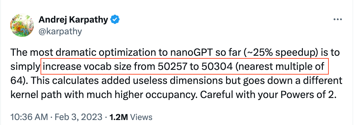
因为这类尺寸通常更符合现代的GPU和CUDA kernel的实现习惯,主要有以下几个好处:
- 更好的Warp 利用:GPU中的线程是以Warp为单位进行调度的,通常一个Warp包含32个线程。如果模型的维度是32的倍数,那么每个Warp都可以被完全利用,避免了资源的浪费。
- CUDA Kernel优化:很多CUDA kernel在处理特定尺寸的数据时会有优化,比如当输入的维度是32、64、128等时,CUDA kernel可以更高效地进行计算,减少内存访问的开销。
- 更适合显存访问:GPU 读取显存不是一个元素一个元素慢慢读,而是按固定大小的 memory segment 来取数据。
- Tensor Core优化:对于NVIDIA的Tensor Core来说,通常要求输入的维度是8、16、32等特定的倍数,这样才能充分利用Tensor Core的计算能力。如果不满足这些条件,则可能无法使用Tensor Core,导致性能下降。
3.3 RoPE Position Embedding
有了Word Embedding Layer之后,我们就需要引入位置信息了。由于Transformer模型没有循环结构,因此需要通过位置编码来引入位置信息,使模型能够理解输入序列中各个元素的相对位置。传统的Transforme(Vaswani et al. 2023)使用的是Sinusoidal Position Encoding,但是在现代的LLM中,我们通常会使用RoPE(Rotary Position Embedding)(Su et al. 2023)来替代传统的Sinusoidal Position Encoding,RoPE是一种基于旋转的位置信息编码方法,它通过对输入的Token向量进行旋转来引入位置信息。具体来说,RoPE将hidden state分成两个一组,然后对每一组进行旋转,旋转的角度由位置信息和hidden state 的维度决定。这样,模型就可以通过旋转后的向量来捕捉输入序列中各个元素的相对位置关系
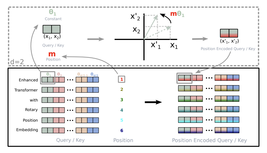
用数学公式表示就是:
\[ RoPE(x, m) = \begin{pmatrix} x_1 \\ x_2 \\ x_3 \\ x_4 \\ \vdots \\ x_{d-1} \\ x_d \end{pmatrix} \otimes \begin{pmatrix} \cos m\theta_1 \\ \cos m\theta_1 \\ \cos m\theta_2 \\ \cos m\theta_2 \\ \vdots \\ \cos m\theta_{d/2} \\ \cos m\theta_{d/2} \end{pmatrix} + \begin{pmatrix} -x_2 \\ x_1 \\ -x_4 \\ x_3 \\ \vdots \\ -x_d \\ x_{d-1} \end{pmatrix} \otimes \begin{pmatrix} \sin m\theta_1 \\ \sin m\theta_1 \\ \sin m\theta_2 \\ \sin m\theta_2 \\ \vdots \\ \sin m\theta_{d/2} \\ \sin m\theta_{d/2} \end{pmatrix} \tag{1}\]
我们可以看到,其中\((x_1, x_2)\)是一组,\((x_3, x_4)\)是一组,以此类推,每一组都会被旋转,旋转的角度由位置信息\(m\)和hidden state的维度决定。通过这种方式,RoPE能够引入位置信息,使模型能够捕捉输入序列中各个元素的相对位置关系,从而提高模型的性能和表达能力。其中\(\theta_i\) 是一个预定义的频率,通常是根据hidden state的维度来计算的,具体来说,\(\theta_i\) 的计算方式如下:
\[ \theta_i = \frac{1}{\text{base}^{2i/d}} \tag{2}\]
其中,\(i\) 是hidden state的维度索引,\(d\) 是hidden state的总维度,\(\text{base}\) 是一个预定义的常数,通常取值为10,000。base的作用是控制控制 RoPE 中各个维度旋转频率的尺度范围,简单来说就是:
- base 大:更多低频,旋转更慢,更偏向长距离
- base 小:更多高频,旋转更快,更偏向短距离
在我们这个项目中,我们会使用默认的base值100,000来计算RoPE的位置编码,这样可以在处理不同长度的输入序列时都能够有较好的性能表现。
我们来看一下如何用代码来实现:
chat_llm/model/llm.py
def apply_rotary_embedding(x: torch.Tensor, cos: torch.Tensor, sin: torch.Tensor) -> torch.Tensor:
    """
    x = cos * x
    """
    assert x.ndim == 4, "Input tensor must be of shape (batch_size, seq_len, num_heads, head_dim)"
    assert cos.shape == sin.shape, "Cosine and sine tensors must have the same shape"
    assert cos.ndim == 4 and sin.ndim == 4, (
        "Cosine and sine tensors must be of shape (1, seq_len, num_heads, head_dim // 2)"
    )

    x1, x2 = x.chunk(2, dim=-1)

    y1 = x1 * cos + x2 * sin
    y2 = x1 * (-sin) + x2 * cos
return torch.cat([y1, y2], dim=-1)接下来,我们看一下如何计算cosine和sine的值,这些值是根据位置信息\(m\)和hidden state的维度来计算的,具体代码如下:
chat_llm/model/llm.py
def pre_compute_cos_sin(
    max_seq_len: int,
    head_dim: int,
    base: int = 100_000,
    device: torch.device = torch.device("cpu"),
    dtype: torch.dtype = torch.float32,
) -> tuple[torch.Tensor, torch.Tensor]:
    channel_range = torch.arange(0, head_dim, 2, device=device, dtype=torch.float32) # Hidden state的维度索引,步长为2,因为每两维为一组

    inv_freq = 1.0 / (base ** (channel_range / head_dim)) # Theta_i的计算方式
    pos_ids = torch.arange(max_seq_len, device=device, dtype=torch.float32) # m 的位置索引

    freqs = torch.einsum("i,j->ij", pos_ids, inv_freq)  # (max_seq_len, head_dim // 2)
    cos, sin = freqs.cos(), freqs.sin()  # (max_seq_len, head_dim // 2)
    cos, sin = cos.to(dtype=dtype), sin.to(dtype=dtype)
    cos = cos[None, :, None, :]  # (1, max_seq_len, 1, head_dim // 2)
    sin = sin[None, :, None, :]  # (1, max_seq_len, 1, head_dim // 2)
    return cos, sin
chat_llm/model/llm.py
class LLMModel(nn.Module):
    def __init__(self, config: ModelConfig, padded_vocab_size: int = 64):
        super().__init__()
        ...
        self.rotary_seq_len = config.max_seq_len * 10
        cos, sin = pre_compute_cos_sin(
            max_seq_len=self.rotary_seq_len,
            head_dim=config.head_dim,
            device=config.device,
            dtype=config.dtype
        )
        self.register_buffer("cos", cos, persistent=False)
        self.register_buffer("sin", sin, persistent=False)
        ...
我们通过 pre_compute_cos_sin 函数来预计算cosine和sine的值,并将其注册为模型的buffer,这样在模型的训练和推理过程中,我们就可以直接使用这些预计算的值来进行RoPE的位置编码了,并且保存为模型状态的一部分,但不需要加载到Optimizer中。
NOTE: Different between code and math equation
细心的读者可能会发现,我们代码的实现和我们上面给出的数学公式有一些不同,根据代码的实现方式,RoPE的配对方式是:\((x_0,x_{d/2}), (x_1,x_{d/2+1}), \dots, (x_{d/2-1},x_{d-1})\), 并且旋转的角度是\(\begin{pmatrix} \cos(m\theta_i) & -\sin(m\theta_i)\\ \sin(m\theta_i) & \cos(m\theta_i) \end{pmatrix}\),而我们上面给出的数学公式中,配对方式是\((x_1,x_2), (x_3,x_4), \dots, (x_{d-1},x_d)\),并且旋转的角度是\(\begin{pmatrix}\cos(m\theta_i) & \sin(m\theta_i)\\ -\sin(m\theta_i) & \cos(m\theta_i) \end{pmatrix}\)。
实际代码实现对应的数学公式:
\[ \mathrm{RoPE}_{\text{code}}(x,m)= \begin{pmatrix} x_1\\ x_2\\ x_3\\ \vdots\\ x_{d/2}\\ x_{d/2+1}\\ x_{d/2+2}\\ x_{d/2+3}\\ \vdots\\ x_d \end{pmatrix} \otimes \begin{pmatrix} \cos m\theta_1\\ \cos m\theta_2\\ \cos m\theta_3\\ \vdots\\ \cos m\theta_{d/2}\\ \cos m\theta_1\\ \cos m\theta_2\\ \cos m\theta_3\\ \vdots\\ \cos m\theta_{d/2} \end{pmatrix} + \begin{pmatrix} x_{d/2+1}\\ x_{d/2+2}\\ x_{d/2+3}\\ \vdots\\ x_d\\ -x_1\\ -x_2\\ -x_3\\ \vdots\\ -x_{d/2} \end{pmatrix} \otimes \begin{pmatrix} \sin m\theta_1\\ \sin m\theta_2\\ \sin m\theta_3\\ \vdots\\ \sin m\theta_{d/2}\\ \sin m\theta_1\\ \sin m\theta_2\\ \sin m\theta_3\\ \vdots\\ \sin m\theta_{d/2} \end{pmatrix} \]
这样实现的好处是:
- 代码更加的简单
- 内存访问更加的连续,效率更高
- Fused Kernel的实现更加的简单
至于为什么用逆时针来旋转,还是顺时针来旋转,这个其实并没有什么区别,主要是一个约定俗成的问题,RoPE的原论文(Su et al. 2023)中是使用逆时针旋转的,我们这里使用顺时针旋转的实现方式,主要是为了代码的简洁性和效率,毕竟在实际的实现中,这两种方式是等价的,并不会对模型的性能和表达能力产生实质性的影响。
另外需要一个注意的点就是,我们把RoPE的位置编码的长度设置为 config.max_seq_len * 10,也就是说,我们预计算了10倍于最大序列长度的RoPE位置编码,这样做的主要目的是提前缓存更长范围的位置编码,从而避免在推理阶段处理更长上下文时重新计算 RoPE 参数。如果后续推理长度超过训练长度,也可以直接复用这部分预计算结果。不过,这并不意味着模型一定具备良好的长上下文外推能力。
3.4 Normalization
在Transformer模型中,Normalization是一个非常重要的组件,它能够帮助模型更好地训练和收敛。传统的Transformer使用的是LayerNorm来进行Normalization,但是在现代的LLM中,我们通常会使用RMSNorm(Zhang and Sennrich 2019)来替代传统的LayerNorm,RMSNorm是一种基于均方根的Normalization方法,它通过计算输入的均方根来进行Normalization,从而提高模型的效率和性能。具体来说,RMSNorm的数学表达式如下:
\[ \mathrm{RMSNorm}(x) = \frac{x}{\sqrt{\frac{1}{d} \sum_{i=1}^{d} x_i^2 + \epsilon}} \tag{3}\] 其中,\(x\) 是输入的向量,\(d\) 是输入向量的维度,\(\epsilon\) 是一个小的常数,用于防止除以零。RMSNorm通过计算输入的均方根来进行Normalization,这样可以避免LayerNorm中计算均值和方差的开销,从而提高模型的效率和性能。并且我们丢掉了RMSNorm中的Learnable Parameters,因为在LLM的训练中, Norm 的主要任务是保持数值的稳定性,而不是学习表达能力,丢掉Learnable Parameters可以进一步减少模型的参数量和计算复杂度。
chat_llm/model/llm.py
3.4.1 Pre-Normalization
在 LLM 训练中,Normalization 的位置也是一个非常重要的设计选择,常见的方式主要有两种:
- Pre-Normalization(Pre-Norm):在每个 Transformer 子层(如 Attention 或 MLP)输入之前进行 Normalization。
- Post-Normalization(Post-Norm):在每个 Transformer 子层输出之后,并在 Residual Add 之后进行 Normalization。
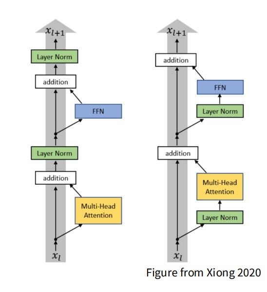
在最初的 Transformer(Vaswani et al. 2023) 中,采用的是 Post-Norm 的设计;而在现代 LLM 中,更常见的是 Pre-Norm。这是因为 Pre-Norm 通常能够带来更好的训练稳定性,尤其是在模型层数较深时表现更明显。
具体来说,Pre-Norm 会将每个子层写成:
\[ x_{l+1} = x_l + F(\mathrm{Norm}(x_l)) \tag{4}\]
而 Post-Norm 的形式通常为: \[ x_{l+1} = \mathrm{Norm}(x_l + F(x_l)) \tag{5}\]
相比之下,Pre-Norm 的 Residual 路径更加“干净”,恒等映射 \(x_l \to x_{l+1}\) 更容易保留下来,因此梯度可以更直接地沿着 Residual Connection (He et al. 2015) 向前传播。这使得深层网络在训练时更不容易出现梯度消失或梯度爆炸的问题,也因此成为现代大规模语言模型中的主流选择。
除了在每个Layer之前加上Normalization,我们还可以在Query和Key的计算中加上Normalization,这也就是所谓的QK-Norm,在之后的Attention Mechanism中,我们会介绍QK-Norm的细节和实现方式。
3.5 Attention Mechanism
接下来,我们来介绍Transformer LM中最复杂的一个组件,也就是Attention Mechanism。在Transformer LM中,用的是Global Attention,时间复杂度为 \(\mathcal{O}(n^2)\),其中\(n\)是输入序列的长度。Global Attention能够捕捉输入序列中各个元素之间的全局依赖关系,从而提高模型的性能和表达能力。但是,Global Attention的计算复杂度较高,当输入序列较长时,计算资源的消耗也会大幅增加。为了解决这个问题,我们可以引入Sliding Window Attention来替代Global Attention,Sliding Window Attention能够捕捉输入序列中各个元素之间的局部依赖关系,从而提高模型的效率和性能。但是,Sliding Window Attention无法捕捉输入序列中各个元素之间的全局依赖关系,从而可能会降低模型的性能和表达能力。为了解决这个问题,我们可以结合Global Attention和Sliding Window Attention来提高模型的效率和性能,这也就是所谓的Hybird Attention。接下来我们来看一下不同的Attention的实现,并且介绍Attention机制中运用到的其他技术细节。
首先看一下Causal Attention层的实现:
chat_llm/model/llm.py
class CausalSelfAttention(nn.Module):
    def __init__(self, config: ModelConfig, layer_idx: int):
        """
        layer_idx:
            1. Determined wether use full context attention of sliding window attention
            2. Used for KV caching in the future
            3. Determined wether use value embeddings
        """
        super().__init__()

        self.layer_idx = layer_idx
        self.n_q_heads = config.n_q_heads
        self.n_kv_heads = config.n_kv_heads

        assert config.embed_dim % self.n_q_heads == 0, "embed_dim must be divisible by n_q_heads"
        self.head_dim = config.embed_dim // self.n_q_heads
        assert self.n_q_heads % self.n_kv_heads == 0, "n_q_heads must be divisible by n_kv_heads"

        self.q_proj = Linear(config.embed_dim, config.n_q_heads * self.head_dim, bias=False)
        self.k_proj = Linear(config.embed_dim, config.n_kv_heads * self.head_dim, bias=False)
        self.v_proj = Linear(config.embed_dim, config.n_kv_heads * self.head_dim, bias=False)
        self.out_proj = Linear(config.n_q_heads * self.head_dim, config.embed_dim, bias=False)

        # Value Embeddings
        self.ve_gate_channels = 12
        self.ve_gate = (
            Linear(self.ve_gate_channels, self.n_kv_heads, bias=False)
            if has_ve(layer_idx, config.n_layers)
            else None
        )

    def forward(
        self,
        x: torch.Tensor,
        ve: torch.Tensor | None,
        cos: torch.Tensor,
        sin: torch.Tensor,
        window_size: int,
        kv_cache,
    ) -> torch.Tensor:
        B, T, C = x.shape

        q = self.q_proj(x).view(B, T, self.n_q_heads, self.head_dim)
        k = self.k_proj(x).view(B, T, self.n_kv_heads, self.head_dim)
        v = self.v_proj(x).view(B, T, self.n_kv_heads, self.head_dim)

        if ve is not None and self.ve_gate is not None:
            ve = ve.view(B, T, self.n_kv_heads, self.head_dim)
            gate = 3 * F.sigmoid(self.ve_gate(x[..., : self.ve_gate_channels]))  # (B, n_kv_heads
            v = v + gate.unsqueeze(-1) * ve

        # Apply rotary embeddings to q and k
        q = apply_rotary_embedding(q, cos, sin)
        k = apply_rotary_embedding(k, cos, sin)

        # Apply QK-Norm
        q = rms_norm(q)
        k = rms_norm(k)
        q = q * 1.15
        k = k * 1.15

        if kv_cache is None:
            out = flash_attn.flash_attn_func(q, k, v, causal=True, window_size=window_size)
        else:
            # Inference with KV caching
            k_cache, v_cache = kv_cache.get_layer_cache(self.layer_idx)
            out = flash_attn.flash_attn_with_kvcache(
                q,
                k_cache,
                v_cache,
                k,
                v,
                cache_seqlens=kv_cache.cache_seq_lens,
                causal=True,
                window_size=window_size,
            )

            if self.layer_idx == kv_cache.n_layers - 1:
                kv_cache.advance(T)

        out = out.contiguous().view(B, T, C)
        out = self.out_proj(out)
        return out
对于每个Attention Layer,我们会保存 layer_idx,这个参数主要有三个作用:
- 根据
layer_idx来确定我们是使用全局注意力(Global Attention)还是滑动窗口注意力(Sliding Window Attention)。 - 在后续的推理阶段,我们会使用KV缓存来加速模型的推理过程,
layer_idx可以帮助我们在KV缓存中正确地存储和访问每一层的Key和Value。 - 根据
layer_idx来确定我们是否使用Value Embeddings,这是一种增强模型表达能力的技术。
3.5.1 Globel Attention
3.5.2 Sliding Window Attention
3.5.3 Hybrid Attention
在LLM的训练中,我们通常会使用Global Attention和Sliding Window Attention的结合来提高模型的效率和性能。Global Attention能够捕捉输入序列中各个元素之间的全局依赖关系,而Sliding Window Attention能够捕捉输入序列中各个元素之间的局部依赖关系。通过结合Global Attention和Sliding Window Attention,我们可以同时捕捉输入序列中各个元素之间的全局依赖关系和局部依赖关系,从而提高模型的效率和性能。
3.6 Feed-Forward Network (FFN)
在模型中,另一个核心组件是 Feed-Forward Network (FFN)。它通常位于每个 Transformer Block 的 Attention 之后,对每个位置的表示独立地进行非线性变换,从而进一步提升模型的表达能力。
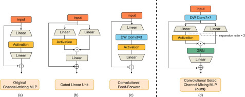
在这里,我们使用的是现代 LLM 中非常常见的一种 FFN 变体,也就是 Gated MLP,更具体地说,可以看作是 SwiGLU 风格 的实现。相比传统 Transformer 中使用的两层 MLP:
\[ \mathrm{FFN}(x) = W_2 \,\sigma(W_1 x) \tag{6}\]
Gated MLP 会额外引入一个门控分支,通过门控机制动态控制信息流动,其形式可以写成:
\[ \mathrm{MLP}(x) = W_{\text{down}}\Big( \mathrm{silu}(W_{\text{gate}}x) \odot (W_{\text{up}}x) \Big) \tag{7}\]
其中:
- \(W_{\text{gate}}\) 对应 gate_proj
- \(W_{\text{up}}\) 对应 up_proj
- \(W_{\text{down}}\) 对应 down_proj
- \(\odot\) 表示逐元素相乘
chat_llm/model/llm.py
class MLP(nn.Module):
    def __init__(self, config):
        super().__init__()
        self.gate_up_proj = Linear(config.embed_dim, 2 * config.d_ff, bias=False)
        self.down_proj = Linear(config.d_ff, config.embed_dim, bias=False)

    def forward(self, x):
        gate, up = self.gate_up_proj(x).chunk(2, dim=-1)
        return self.down_proj(F.silu(gate) * up)
有一个需要注意的点就是,在这个实现中,我们将 gate_proj 和 up_proj 合并成了一个线性层 gate_up_proj,\([x_{\text{gate}}, x_{\text{up}}] = W_x\),这样可以减少一次矩阵乘法的计算。
3.7 Attention Residual
3.8 Dummy Test
4 Optimizer
4.1 AdamW
4.2 Muon
4.3 ZeRO-2
5 Tokenizer
6 Dataset & DataLoader
7 Scaling Laws
8 Pre-Training Evaluateion Metrics
9 Pre-Training
9.1 Mixed Precision Training
9.2 Gradient Accumulation
10 Instruction-Tuning (SFT)
在我们Pre-Training结束之后,我们得到了一个基础的LLM,这个语言模型可以做词语接龙,比如:
猫猫是一个 猫猫是一个很 猫猫是一个很可 猫猫是一个很可爱…
这距离我们的ChatGPT-Style LLM的目标还有一段距离,我们需要让模型可以输出特定的格式,能够理解指令,并且能够对话生成。为此,我们需要进行Instruction-Tuning,也就是SFT(Supervised Fine-Tuning)。我们会使用一些公开的指令数据集,比如Alpaca、ShareGPT等,来对模型进行微调,让它能够更好地理解和执行各种指令。
10.1 Dataset Preparation
10.1.1 Basic Task
10.1.2 SmolTalk
10.1.3 Arc
10.1.4 MMLU
10.1.5 GSM8K
10.1.6 Customized Instruction Dataset
除了上述的公开集,我们还可以自己构建一些
11 Post-Training (GRPO)
12 Gradio Chat Interface
13 Conclusion
14 What’s Next
完成了这个Project之后,我们真正的理解了如何从0训练一个ChatGPT-Style的LLM系统,基本上市面上所有的SOTA的模型,都是基于这一套技术。当然,学无止境,在这个项目的基础上,我们还有很多可以继续深入的方向:
- AutoResearch:Karpathy大神开源的AutoResearch工具,可以自动迭代模型结构、优化器、超参数等,来找到最优的训练方案。
- Multi-Modality LLM:目前我们训练的模型主要是基于文本的,但未来我们可以尝试训练一个多模态的LLM,能够处理图像、视频、音频等多种输入形式。
- Inference Optimization:优化模型的推理过程
- Reasoning Capabilities:尽管我们实现了GRPO的算法,但是模型的推理能力还有很大的提升空间,比如我们可以尝试新的推理算法,或者引入别的训练数据。
14.1 AutoResearch
在这个nanoChat项目之后,Karpathy大神有开源了一个叫做AutoResearch的神器(GitHub上的Stars比这个项目还高),它通过定义简单的三个文件:
prepare.py:数据准备脚本train.py:训练脚本program.md: 告诉Agent该怎么做
通过这个方法,Agent自动迭代模型结构、优化器、超参数、训练循环、batch size、model size 等等,来找到最优的训练方案。不过我觉得最有创新的方法就是它可以通过git来回滚,保留好的结果,回滚坏的结果。通过这种方式,AutoResearch可以在没有人类干预的情况下自动进行实验和优化,并提高了模型的性能,如下图所示:

14.2 Multi-Modality LLM
基于文本的LLM已经非常强大了,但未来我们可以尝试训练一个多模态的LLM,能够处理图像、视频、音频等多种输入形式。比如我们可以训练一个模型,输入一张图片,它能够生成对这张图片的描述,或者输入一段视频,它能够总结视频的内容,甚至输入一段音频,它能够转录成文本并进行分析。常见的MLLM的框架有:
- LLaVA
14.3 Inference System
15 In the end
创作不易,如果你觉得内容对你有帮助,欢迎请我 喝杯咖啡/支付宝红包,支持我继续创作!你们的支持是我最大的动力! :)