PaliGemma Inference and LoRA Fine Tuning
LoRA, PyTorch, Gradio, Grouped Query Attention, RoPE, KV Cache
Hi everyone! In this project, we will explore the PaliGemma (Beyer et al. 2024) model, a multi-modal large language model that combines vision and language tasks. PaliGemma model is an open-source model developed by the Pali Research Community, designed to handle both image and text inputs effectively. We choose this project as starting point to understand the capabilities of multi-modal models and how to fine-tune them for specific applications. Without further talking, let’s dive in!
1 Preliminaries
Before we start, make sure you have the following prerequisites installed:
It will install all the necessary libraries and dependencies required for this project.
To better understand the PaliGemma model, we need understand the following models:
- Trasnformer(Vaswani et al. 2023) Architecture: [My Blog][My Implementation]
- Vision Transformer (ViT)(Dosovitskiy et al. 2021): [My Blog][My Implementation]
- CLIP (Radford et al. 2021): [My Blog][My Implementation]
If you are not familiar with these models, I highly recommend checking out the provided blog posts and implementations before proceeding with this project.
With the preliminaries covered, we can now move on to exploring the PaliGemma model itself.
2 PaliGemma Model Overview
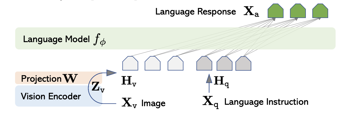
PaliGemma is a multi-modal large language model that integrates vision and language tasks. It fusion the Image and Text through LLaVA(Liu et al. 2023) architecture, the architecure consists of three main components:
- Vision Encoder: An model encoder image into feature representations.
- Projector Layer: A linear layer that projects the image features into a text-compatible space.
- Language Model: A large language model (LLM) that processes the combined image and text features to generate responses.
The overall architecture architecure of LLaVA is illustrated below:
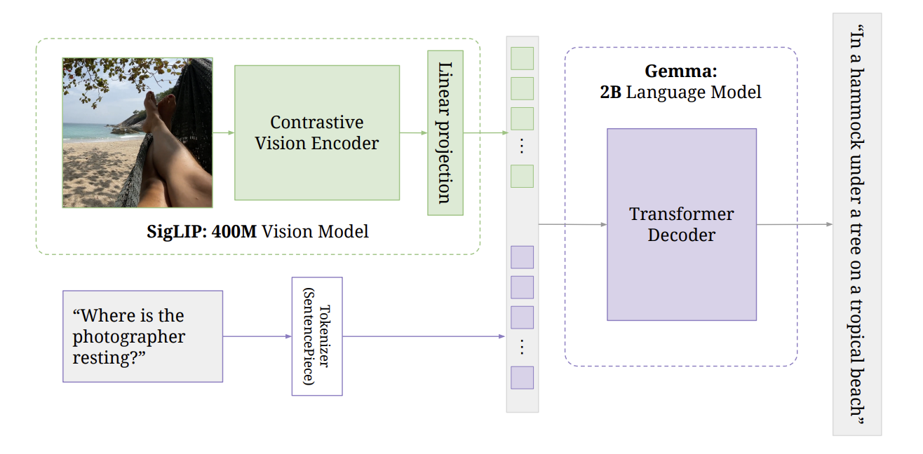
Base on the LLaVA architecture, PaliGemma has the same architecture but uses different pre-trained models for the vision encoder and language model. Specifically, PaliGemma uses the following pre-trained models:
- Vision Encoder: Vision Trasnformer model pre-trained used in SigLIP
- Language Model: Gemma 2B model
- Projector Layer: A linear layer that maps the vision encoder output to the language model input space.
The overall architecture of PaliGemma is illustrated below:
Has been understood the overall architecture of PaliGemma, let’s dig into each compoent in more details. First, we will explore the Vision Encoder.
2.1 Vision Encoder
The vision encoder in PaliGemma is based on the Vision Transformer (ViT) (Dosovitskiy et al. 2021) architecture. The following figure illustrates the architecture of the Vision Transformer:

It start with the patch embedding layer, which splits the input image into fixed-size patches and linearly embeds them into a sequence of vectors.:
class SiglipVisionEmbeddings(nn.Module):
    def __init__(self, config: ModelConfig):
        super().__init__()

        self.embed_dim = config.vision_hidden_size
        self.image_size = config.vision_image_size
        self.patch_size = config.vision_patch_size

        self.patch_embedding = nn.Conv2d(
            in_channels=config.vision_num_channels,
            out_channels=config.vision_hidden_size,
            kernel_size=config.vision_patch_size,
            stride=config.vision_patch_size,
            padding="valid",
        )

        ...

    def forward(self, imgs: torch.Tensor) -> torch.Tensor:
        patch_embeds = self.patch_embedding(imgs)
        patch_embeds = patch_embeds.flatten(2).transpose(1, 2)

        ...
After obtaining the patch embeddings, position embeddings are added to retain spatial information. Here we combine the patch embeddings with position embeddings:
class SiglipVisionEmbeddings(nn.Module):
    def __init__(self, config: ModelConfig):
        super().__init__()

        self.embed_dim = config.vision_hidden_size
        self.image_size = config.vision_image_size
        self.patch_size = config.vision_patch_size

        self.patch_embedding = nn.Conv2d(
            in_channels=config.vision_num_channels,
            out_channels=config.vision_hidden_size,
            kernel_size=config.vision_patch_size,
            stride=config.vision_patch_size,
            padding="valid",
        )

        assert self.image_size % self.patch_size == 0, "Image size must be divisible by patch size"
        num_patches = (self.image_size // self.patch_size) ** 2
        self.num_positions = num_patches
        self.position_embedding = nn.Embedding(self.num_positions, self.embed_dim)
        self.register_buffer(
            "position_ids",
            torch.arange(self.num_positions, dtype=torch.int64).expand((1, -1)),
            persistent=False,
        )

    def forward(self, imgs: torch.Tensor) -> torch.Tensor:
        patch_embeds = self.patch_embedding(imgs)
        patch_embeds = patch_embeds.flatten(2).transpose(1, 2)

        position_embeds = self.position_embedding(self.position_ids)

        return patch_embeds + position_embeds
After get the combined embeddings, they are fed into a series of transformer encoder layers to capture global dependencies and extract high-level features from the image. The transformer encoder consists of multiple layers of multi-head self-attention and feed-forward neural networks.
class SiglipAttention(nn.Module):
    def __init__(self, config: ModelConfig):
        super().__init__()

        self.embed_dim = config.vision_hidden_size
        self.num_heads = config.vision_num_attention_heads

        assert self.embed_dim % self.num_heads == 0, (
            "Embedding dimension must be divisible by number of heads"
        )
        self.head_dim = self.embed_dim // self.num_heads

        self.q_proj = nn.Linear(self.embed_dim, self.embed_dim)
        self.k_proj = nn.Linear(self.embed_dim, self.embed_dim)
        self.v_proj = nn.Linear(self.embed_dim, self.embed_dim)
        self.out_proj = nn.Linear(self.embed_dim, self.embed_dim)

        self.dropout_prob = config.vision_attention_dropout

    def forward(self, hidden_states: torch.Tensor) -> tuple[torch.Tensor, torch.Tensor]:
        B, S, D = hidden_states.shape

        q = self.q_proj(hidden_states).view(B, S, self.num_heads, self.head_dim).transpose(1, 2)
        k = self.k_proj(hidden_states).view(B, S, self.num_heads, self.head_dim).transpose(1, 2)
        v = self.v_proj(hidden_states).view(B, S, self.num_heads, self.head_dim).transpose(1, 2)

        attn_weights = (q @ k.transpose(-2, -1)) * self.head_dim**-0.5
        attn_weights = attn_weights.softmax(dim=-1)

        if self.dropout_prob > 0:
            attn_weights = nn.functional.dropout(attn_weights, p=self.dropout_prob, training=self.training)

        attn_output = (attn_weights @ v).transpose(1, 2).contiguous().view(B, S, D)

        attn_output = self.out_proj(attn_output)

        return attn_output, attn_weights
And the feed forward network is defined as follows:
class SiglipMLP(nn.Module):
    def __init__(self, config: ModelConfig):
        super().__init__()

        self.fc1 = nn.Linear(config.vision_hidden_size, config.vision_intermediate_size)
        self.fc2 = nn.Linear(config.vision_intermediate_size, config.vision_hidden_size)

    def forward(self, hidden_states: torch.Tensor) -> torch.Tensor:
        hidden_states = self.fc1(hidden_states)
        hidden_states = F.gelu(hidden_states, approximate="tanh")
        hidden_states = self.fc2(hidden_states)

        return hidden_states
The complete transformer encoder layer combines the attention and feed-forward network as follows:
class SiglipEncoderLayer(nn.Module):
    def __init__(self, config: ModelConfig):
        super().__init__()

        self.self_attn = SiglipAttention(config)
        self.layer_norm1 = nn.LayerNorm(config.vision_hidden_size, eps=config.vision_layer_norm_eps)

        self.mlp = SiglipMLP(config)
        self.layer_norm2 = nn.LayerNorm(config.vision_hidden_size, eps=config.vision_layer_norm_eps)

    def forward(self, hidden_states: torch.Tensor) -> torch.Tensor:
        residual = hidden_states
        hidden_states = self.layer_norm1(hidden_states)
        attn_output, _ = self.self_attn(hidden_states)
        hidden_states = residual + attn_output

        residual = hidden_states
        hidden_states = self.layer_norm2(hidden_states)
        mlp_output = self.mlp(hidden_states)
        hidden_states = residual + mlp_output

        return hidden_states
In each transformer encoder layer, we first apply layer normalization(Ba, Kiros, and Hinton 2016) to the input hidden states. Then, we compute the self-attention output using the SiglipAttention module. The attention output is added to the residual connection(He et al. 2015) to form the updated hidden states.
Stack multiple transformer encoder layers to form the complete vision encoder:
class SiglipEncoder(nn.Module):
    def __init__(self, config: ModelConfig):
        super().__init__()

        self.layers = nn.ModuleList(
            [SiglipEncoderLayer(config) for _ in range(config.vision_num_hidden_layers)]
        )

    def forward(self, inputs_embeds: torch.Tensor) -> torch.Tensor:
        hidden_states = inputs_embeds
        for layer in self.layers:
            hidden_states = layer(hidden_states)

        return hidden_states
Finally, we define the complete vision encoder by combining the patch embedding, position embedding, and transformer encoder:
class SiglipVisionTransformer(nn.Module):
    def __init__(self, config: ModelConfig):
        super().__init__()

        self.embeddings = SiglipVisionEmbeddings(config)
        self.encoder = SiglipEncoder(config)

        self.post_layernorm = nn.LayerNorm(config.vision_hidden_size, eps=config.vision_layer_norm_eps)

    def forward(self, imgs: torch.Tensor) -> torch.Tensor:
        hidden_states = self.embeddings(imgs)
        hidden_states = self.encoder(hidden_states)
        hidden_states = self.post_layernorm(hidden_states)
        return hidden_states
With the following vision encoder configuration:
@dataclass
class ModelConfig:
    # Vision Configuration
    vision_num_channels: int = 3
    vision_image_size: int = 224
    vision_patch_size: int = 14
    vision_num_image_tokens: int = 256
    vision_hidden_size: int = 1152
    vision_intermediate_size: int = 4304
    vision_num_hidden_layers: int = 27
    vision_num_attention_heads: int = 16

    vision_layer_norm_eps: float = 1e-6
    vision_attention_dropout: float = 0.0

    ...
let’s walk through an example of how to use the vision encoder to process an input image:
- Load and preprocess the input image to match the expected input size of the vision encoder \((3, 224, 224)\).
- Pass the preprocessed image through the patch embedding and position embedding layers to obtain the combined embeddings with shape \((1, 256, 1152)\), where \(224 / 14 = 16\) patches along each dimension, resulting in \(16 \times 16 = 256\) patches.
- Feed the combined embeddings into the transformer encoder, which consists of 27 layers of multi-head self-attention and feed-forward networks.
- The output of the vision encoder will be a tensor of shape \((1, 256, 1152)\), representing the high-level feature representations extracted from the input image.
\[ (1, 3, 224, 224) \xrightarrow{\text{Vision Embedding}} (1, 256, 1152) \xrightarrow{\text{Encoding}} (1, 256, 1152) \tag{1}\]
This is same for all input images, regardless of their content. The vision encoder processes the image to extract meaningful features that can be used for downstream tasks.
2.1.1 Aside: How Vision Transformer trained?
The ViT used in the PaliGemma model is pre-trained using SigLIP method, which is a variant of CLIP(Radford et al. 2021) specifically designed for vision transformers. Here is the overview of CLIP training process:
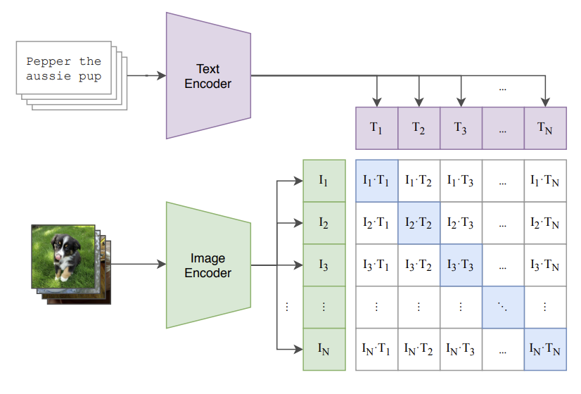
CLIP optimize the model using contrastive loss function:
\[ \mathcal{L}_{CLIP} = - \frac{1}{N} \sum_{i=1}^{N} \left[ \log \frac{\exp(\text{sim}(f_{\text{img}}(x_i), f_{\text{text}}(y_i)) / \tau)}{\sum_{j=1}^{N} \exp(\text{sim}(f_{\text{img}}(x_i), f_{\text{text}}(y_j)) / \tau)} + \log \frac{\exp(\text{sim}(f_{\text{text}}(y_i), f_{\text{img}}(x_i)) / \tau)}{\sum_{j=1}^{N} \exp(\text{sim}(f_{\text{text}}(y_i), f_{\text{img}}(x_j)) / \tau)} \right] \tag{2}\]
However, SigLIP change the training objective to focus on image-image similarity instead of image-text similarity. This is achieved by using a dataset of image pairs that are semantically similar, and optimizing the model to maximize the similarity between these pairs.
So, the SigLIP is best suited for tasks that require strong visual understanding, such as image classification, object detection, and image retrieval. This makes it a good fit for the vision encoder in PaliGemma, which needs to effectively process and understand images in conjunction with text inputs.
2.2 Language Model
The language model in PaliGemma is based on the Gemma 2B model. It is a transformer-based language model that can process text inputs and generate coherent responses. The architecture of the Gemma 2B model is similar to other transformer-based language models such as LLaMA(Touvron et al. 2023) and GPT (Radford et al., n.d.), consisting of multiple layers of self-attention and feed-forward neural networks.
Let’s define the components of the Gemma 2B language model from bottom up. The first, without doublt,is the word embedding layer, which maps input tokens to dense vector representations:
class GemmaModel(nn.Module):
    def __init__(self, config):
        super().__init__()

        self.embed_tokens = nn.Embedding(config.vocab_size, config.hidden_size)

        ...

    def get_input_embeddings(self):
        return self.embed_tokens
One thing to notice is that, unlike other Uni-model LLMs, we DO NOT pass the text input directly to the language model. Instead, we first combine the text embeddings with the image features from the vision encoder through a projector layer. We will save those combination details for later discussion.
The next component is the (causal) self-attention mechanism, which allows the model to attend to different parts of the input sequence when generating responses, with the causal mask ensuring that each token can only attend to previous tokens in the sequence, which provide the autoregressive property:
class GemmaAttention(nn.Module):
    def __init__(self, config: ModelConfig, layer_idx: int):
        super().__init__()
        self.config = config

        self.q_proj = nn.Linear(
            config.lm_hidden_size,
            config.lm_num_heads * config.lm_head_dim,
            bias=config.lm_attention_bias,
        )
        self.k_proj = nn.Linear(
            config.lm_hidden_size,
            config.lm_num_key_value_heads * config.lm_head_dim,
            bias=config.lm_attention_bias,
        )
        self.v_proj = nn.Linear(
            config.lm_hidden_size,
            config.lm_num_key_value_heads * config.lm_head_dim,
            bias=config.lm_attention_bias,
        )
        self.o_proj = nn.Linear(
            config.lm_num_heads * config.lm_head_dim,
            config.lm_hidden_size,
            bias=config.lm_attention_bias,
        )

    def forward(
        self,
        hidden_states: torch.Tensor,
        attention_mask: Optional[torch.Tensor] = None,
        position_ids: Optional[torch.Tensor] = None,
        kv_cache: Optional[KVCache] = None,
        **kwargs,
    ):
        B, S, D = hidden_states.shape
        d_k = D // self.config.lm_num_heads

        q = (
            self.q_proj(hidden_states)
            .view(B, S, self.config.lm_num_heads, self.config.lm_head_dim)
            .transpose(1, 2)
        )

        k = (
            self.k_proj(hidden_states)
            .view(B, S, self.config.lm_num_key_value_heads, self.config.lm_head_dim)
            .transpose(1, 2)
        )

        v = (
            self.v_proj(hidden_states)
            .view(B, S, self.config.lm_num_key_value_heads, self.config.lm_head_dim)
            .transpose(1, 2)
        )

        ...

        attn = torch.matmul(q, k.transpose(-2, -1)) / (d_k**0.5)

        assert attention_mask is not None
        # attn = attn + attention_mask
        attn = attn.masked_fill_(~attention_mask, value=float("-inf"))

        attn = attn.softmax(dim=-1)
        attn = F.dropout(attn, p=self.config.lm_attention_dropout, training=self.training)

        out = torch.matmul(attn, v)
        out = out.transpose(1, 2).contiguous().view(B, S, D)
        out = self.o_proj(out)

        return out, attn
Pretty standard attention mechanism, right? WAIT!! hold on, it that Trasnformer need positional encoding to retain the order information of the input sequence? Where is the positional encoding here? In the Gemma, they use the RoPE (Rotary Position Embedding(Su et al. 2023) technique to encode positional information directly into the attention mechanism. This is done by applying a rotation to the query and key vectors based on their position in the sequence, allowing the model to capture relative positional relationships without explicit positional embeddings. Let’s look at what is the RoPE.
2.2.1 Rotary Position Embedding (RoPE)
Rotary Position Embedding (RoPE) is a technique used to encode positional information directly into the attention mechanism of transformer models. Unlike traditional positional embeddings that are added to the input embeddings(we see ViT is doing this), RoPE applies a rotation to the query and key vectors based on their position in the sequence. This allows the model to capture relative positional relationships more effectively. The rotation matrix is defined as follows:
\[ R(\theta) = \begin{bmatrix}\cos(\theta) & -\sin(\theta) \\\sin(\theta) & \cos(\theta)\end{bmatrix} \tag{3}\]
Where \(\theta\) is the rotation angle determined by the position of the token in the sequence and the dimension of the embedding. The rotation is applied to each pair of dimensions in the query and key vectors with the form \(m\theta_{i}\), where \(m\) is the position index and \(\theta_{i}\) is the base angle for dimension \(i\). The base angle is calculated as follows:
\[ \theta_{i} = \frac{1}{10000^{2i/d}} \tag{4}\]
Each pair of dimensions \((2i, 2i+1)\) in the query and key vectors is rotated using the rotation matrix \(R(\theta_{p,2i})\) and \(R(\theta_{p,2i+1})\). This results in new query and key vectors that incorporate positional information through rotation, so, the final Rotation matrix for the entire embedding dimension can be represented as a block diagonal matrix:
\[ R_p = \begin{bmatrix}R(\theta_{p,0}) & 0 & \cdots & 0 \\ 0 & R(\theta_{p,2}) & \cdots & 0 \\ \vdots & \vdots & \ddots & \vdots \\ 0 & 0 & \cdots & R(\theta_{p,d-2}) \end{bmatrix} \tag{5}\]
However, this is computationally expensive to implement directly. Instead, we can apply the rotation more efficiently using element-wise operations. The rotated query and key vectors can be computed as follows:
\[ R^{d}_{\Theta,m}\,x = \begin{pmatrix} x_{1}\\ x_{2}\\ x_{3}\\ x_{4}\\ \vdots\\ x_{d-1}\\ x_{d} \end{pmatrix} \otimes \begin{pmatrix} \cos(m\theta_{1})\\ \cos(m\theta_{1})\\ \cos(m\theta_{2})\\ \cos(m\theta_{2})\\ \vdots\\ \cos(m\theta_{d/2})\\ \cos(m\theta_{d/2}) \end{pmatrix} \;+\; \begin{pmatrix} -x_{2}\\ x_{1}\\ -x_{4}\\ x_{3}\\ \vdots\\ -x_{d}\\ x_{d-1} \end{pmatrix} \otimes \begin{pmatrix} \sin(m\theta_{1})\\ \sin(m\theta_{1})\\ \sin(m\theta_{2})\\ \sin(m\theta_{2})\\ \vdots\\ \sin(m\theta_{d/2})\\ \sin(m\theta_{d/2}) \end{pmatrix} \tag{6}\]
where \(\otimes\) denotes element-wise multiplication, and \(m\) is the position index. This formulation allows us to efficiently compute the rotated query and key vectors without explicitly constructing the full rotation matrix. Let see how it is implemented in code, first is the inverse frequency calculation:
\[ \text{inv\_freq}[i] = \frac{1}{10000^{2i/d}} \tag{7}\]
Notice that we only compute the inverse frequency for half of the dimensions since each pair of dimensions shares the same base angle. And the shape of inv_freq is (dim/2,). When the forward function is called, with the position_ids provided, we first compute the sinusoidal embeddings:
def forward(self, x, position_ids):
    device = x.device
    dtype = x.dtype

    self.inv_freq = self.inv_freq.to(device)
    inv_freq_expanded = self.inv_freq[None, :, None].float().expand(position_ids.shape[0], -1, 1)
    position_ids_expanded = position_ids[:, None, :].float()

    freqs = (inv_freq_expanded.float() @ position_ids_expanded.float()).transpose(1, 2)
    # emb: [Batch_Size, Seq_Len, Head_Dim]
    emb = torch.cat((freqs, freqs), dim=-1)
    # cos, sin: [Batch_Size, Seq_Len, Head_Dim]
    cos = emb.cos()
    sin = emb.sin()
    return cos.to(dtype=dtype), sin.to(dtype=dtype)
Here, we compute the outer product of the inverse frequencies and position IDs to obtain the rotation angles for each position in the sequence. We then concatenate the angles to create the full embedding and compute the cosine and sine values. These values will be used to rotate the query and key vectors.
By this point, we have obtained the cosine and sine values for the rotations. Next, we apply the rotations to the query and key vectors, first we need to change the x to [-x_2, x_1, -x_4, x_3, ...] format:
def rotate_half(x):
    x1 = x[..., : x.shape[-1] // 2]
    x2 = x[..., x.shape[-1] // 2 :]
    return torch.cat((-x2, x1), dim=-1)
WARNING: About rotate half
One thing to notice and borther me at begin is that, the rotate_half function DOES NOT change the x to [-x_2, x_1, -x_4, x_3, ...] but it change the x to [-x_(d/2+1), -x_(d/2+2), ..., -x_d, x_1, x_2, ..., x_(d/2)] format. We can do this because in the rotate equation, we also concat the \(\theta_i\) as \([\theta_1, \theta_2, \cdots, \theta_{d/2}, \theta_1, \theta_2, \cdots, \theta_{d/2}]\), so this become:
\[ R^{d}_{\Theta,m}\,x = \begin{pmatrix} x_{1}\\ x_{2}\\ x_{3}\\ \vdots\\ x_{d/2}\\ x_{(d/2)+1}\\ x_{(d/2)+2}\\ \vdots\\ x_{d} \end{pmatrix} \otimes \begin{pmatrix} \cos(m\theta_{1})\\ \cos(m\theta_{2})\\ \cos(m\theta_{3})\\ \vdots\\ \cos(m\theta_{d/2})\\ \cos(m\theta_{1})\\ \cos(m\theta_{2})\\ \vdots\\ \cos(m\theta_{d/2}) \end{pmatrix} \;+\; \begin{pmatrix} -x_{(d/2)+1}\\ -x_{(d/2)+2}\\ -x_{(d/2)+3}\\ \vdots\\ -x_{d}\\ x_{1}\\ x_{2}\\ \vdots\\ x_{(d/2)} \end{pmatrix} \otimes \begin{pmatrix} \sin(m\theta_{1})\\ \sin(m\theta_{2})\\ \sin(m\theta_{3})\\ \vdots\\ \sin(m\theta_{d/2})\\ \sin(m\theta_{1})\\ \sin(m\theta_{2})\\ \vdots\\ \sin(m\theta_{d/2}) \end{pmatrix} \]
use \((x_i, x_{i + d/2})\) as the pair for rotation.
We can apply the rotation to the query and key vectors as follows:
2.2.2 Feed Forward Network
After the attention layer, next is the feed forward network, which consists of two linear layers with a GeGLU activation in between. The feed forward network is defined as follows:
\[ \text{FFN(x)} = W_{down} \cdot \big(\text{GELU}(W_{gate} \cdot x) \odot (W_{up} \cdot x)\big) \tag{8}\]
where GELU is the Gaussian Error Linear Unit activation function, defined as:
\[ \text{GELU}(x) = 0.5x \left(1 + \tanh\left(\sqrt{\frac{2}{\pi}} \left(x + 0.044715x^3\right)\right)\right) \tag{9}\]
class GemmaMLP(nn.Module):
    def __init__(self, config: ModelConfig):
        super().__init__()

        self.hidden_size = config.lm_hidden_size
        self.intermediate_size = config.lm_intermediate_size
        self.gate_proj = nn.Linear(self.hidden_size, self.intermediate_size, bias=False)
        self.up_proj = nn.Linear(self.hidden_size, self.intermediate_size, bias=False)
        self.down_proj = nn.Linear(self.intermediate_size, self.hidden_size, bias=False)

    def forward(self, x):
        return self.down_proj(nn.functional.gelu(self.gate_proj(x), approximate="tanh") * self.up_proj(x))
2.2.3 RMSNorm
One last thing in the decoder layer is the normalization layer. In Gemma, they use RMSNorm(Zhang and Sennrich 2019) instead of LayerNorm(Ba, Kiros, and Hinton 2016) for normalization. RMSNorm normalizes the input based on its root mean square (RMS) value, which can be more stable and efficient than traditional layer normalization. The RMSNorm is defined as follows:
\[ \text{RMSNorm}(x) = \frac{x}{\sqrt{\frac{1}{d} \sum_{i=1}^{d} x_i^2 + \epsilon}} \odot g \tag{10}\]
where \(g\) is a learnable scaling parameter, initialized to ones, and \(\epsilon\) is a small constant to prevent division by zero. Here is the implementation of RMSNorm:
class GemmaRMSNorm(nn.Module):
    def __init__(self, dim: int, eps: float = 1e-6):
        super().__init__()

        self.eps = eps
        self.weight = nn.Parameter(torch.zeros(dim))

    def forward(self, x: torch.Tensor) -> torch.Tensor:
        div = torch.rsqrt(torch.sum(x**2, dim=-1, keepdim=True) / x.shape[-1] + self.eps)

        return x * div * (1.0 + self.weight)
NOTE: (1.0 + self.weight) in the RMSNorm
Gemma stores the RMSNorm scale as an offset from 1:
- The forward uses
scale = (1 + weight). weightis initialized to 0, so the initial scale is exactly 1 (identity scale).- This parameterization plays nicer with weight decay / regularization: decay pulls
weight → 0, which keeps the effective scale near 1, instead of pulling a directly-storedgammatoward 0. - It also makes early training more stable because updates change the scale as a small deviation around 1.
So weight=0 + (1+weight) is mainly a stable, optimizer-friendly way to implement “gamma starts at 1”.
2.2.4 Gemma Decoder Layer
Put the attention, rms-norm and feed forward network together to form a transformer decoder layer:
class GemmaDecoderLayer(nn.Module):
    def __init__(self, config: ModelConfig, layer_idx: int):
        super().__init__()
        self.config = config
        self.layer_idx = layer_idx

        self.self_attn = GemmaAttention(config, layer_idx)
        self.input_layernorm = GemmaRMSNorm(config.lm_hidden_size, eps=config.lm_rms_norm_eps)

        self.mlp = GemmaMLP(config)
        self.post_attention_layernorm = GemmaRMSNorm(config.lm_hidden_size, eps=config.lm_rms_norm_eps)

    def forward(
        self,
        hidden_states: torch.Tensor,
        attention_mask: Optional[torch.Tensor] = None,
        position_ids: Optional[torch.Tensor] = None,
        kv_cache: Optional[KVCache] = None,
    ):
        residual = hidden_states
        hidden_states = self.input_layernorm(hidden_states)
        hidden_states, _ = self.self_attn(
            hidden_states,
            attention_mask=attention_mask,
            position_ids=position_ids,
            kv_cache=kv_cache,
        )
        hidden_states = residual + hidden_states

        residual = hidden_states
        hidden_states = self.post_attention_layernorm(hidden_states)
        hidden_states = self.mlp(hidden_states)
        return residual + hidden_states
Similairly, stack multiple decoder layers to form the complete language model decoder:
class GemmaModel(nn.Module):
    def __init__(self, config: ModelConfig):
        super().__init__()
        self.config = config
        self.padding_idx = config.pad_token_id
        self.vocab_size = config.lm_vocab_size

        self.embed_tokens = nn.Embedding(self.vocab_size, config.lm_hidden_size, self.padding_idx)

        self.layers = nn.ModuleList(
            [GemmaDecoderLayer(config, layer_idx) for layer_idx in range(config.lm_num_hidden_layers)]
        )
        self.norm = GemmaRMSNorm(config.lm_hidden_size, eps=config.lm_rms_norm_eps)

    def get_input_embeddings(self):
        return self.embed_tokens

    def forward(
        self,
        attention_mask: torch.Tensor,
        position_ids: torch.Tensor,
        inputs_embeds: torch.Tensor,
        kv_cache: KVCache,
    ):
        # Normalized
        hidden_states = inputs_embeds * (self.config.lm_hidden_size**0.5)

        for decoder_layer in self.layers:
            # [Batch_Size, Seq_Len, Hidden_Size]
            hidden_states = decoder_layer(
                hidden_states,
                attention_mask=attention_mask,
                position_ids=position_ids,
                kv_cache=kv_cache,
            )

        return self.norm(hidden_states)
We add a final RMSNorm layer after the last decoder layer to normalize the output hidden states.
Same as the vision encoder, we define the configuration for the Gemma language model as follows:
@dataclass
class ModelConfig:
    ...

    lm_vocab_size: int = 257216
    lm_hidden_size: int = 2048
    lm_intermediate_size: int = 16384
    lm_num_hidden_layers: int = 18
    lm_num_attention_heads: int = 8
    lm_num_key_value_heads: int = 1
    lm_num_heads: int = 8
    lm_head_dim: int = 256
    lm_max_position_embeddings: int = 8192
    lm_rms_norm_eps: float = 1e-6
    lm_rope_theta: float = 10000.0
    lm_attention_bias: bool = False
    lm_attention_dropout: float = 0.0

    ...
With this config, let’s walk through an example of how to use the Gemma language model to process text inputs:
- Tokenize the input text using a tokenizer compatible with the Gemma model to obtain input token IDs.
- Pass the input token IDs through the embedding layer to obtain input embeddings with shape \((1, L, 2048)\), where \(L\) is the length of the input sequence.
- Pass the input embeddings through the series of decoder layers, each consisting of self-attention and feed-forward networks.
- The output of the language model will be a tensor of shape \((1, L, 2048)\), representing the processed text features.
The concat of the vision encoder and language model happens between step 2 and step 3, which we will discuss in the next section about the projector layer.
2.3 Projector Layer
The projector layer in PaliGemma is a linear layer that maps the output features from the vision encoder to a space compatible with the input of the language model. This is necessary because the dimensions of the vision encoder output and the language model input may differ. The projector layer is defined as follows:
\[ \text{Projector}(x) = W_{p} \cdot x + b_{p} \tag{11}\]
class PaliGemmaMultiModalProjector(nn.Module):
    def __init__(self, config: ModelConfig):
        super().__init__()

        self.linear = nn.Linear(config.vision_hidden_size, config.projection_dim, bias=True)

    def forward(self, x: torch.Tensor) -> torch.Tensor:
        return self.linear(x)
This just a simple linear transformation that adjusts the feature dimensions. When the vision features are passed through the projector layer, they are transformed to match the expected input size of the language model:
\[ (B, 224, D_{vision}) \xrightarrow{\text{Projector}} (B, 224, D_{lm}) \tag{12}\]
in our case, \(D_{vision} = 1152\) and \(D_{lm} = 2048\).
2.4 Putting It All Together: PaliGemma Model
Good, now we have all the components in the Figure 2 assembled. The overall architecture of PaliGemma model can be summarized as follows:
- The input image is processed by the vision encoder (ViT) to extract high-level visual features.
- The extracted visual features are passed through the projector layer to map them to the language model’s input space.
- The input text is tokenized and embedded using the language model’s embedding layer.
- The projected visual features and text embeddings are concatenated to form a combined input sequence for the language model.
- The combined input sequence is processed by the language model (Gemma 2B) to generate coherent text responses.
Here come the most confusion part in the PaliGemma model, the MASK! Let’s see how the attention mask is constructed for the combined input sequence.
2.4.1 Attention Mask Construction
There are three types of mask in the attention mask:
- Causal Mask for decoding the text input.
- Padding Mask for handling variable-length input sequences.
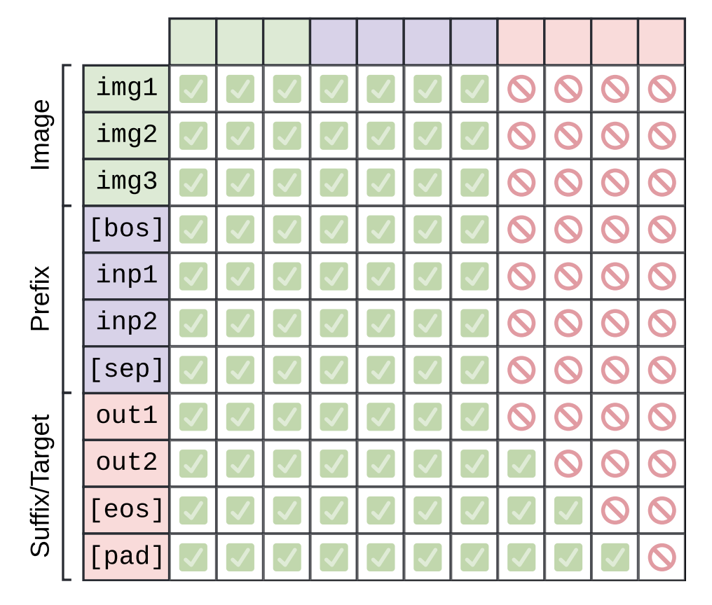
But let’s first see what is the input tokens to the language model look like. Here is the example input sequence:
where IMG_TOKEN_i are placeholder tokens representing the image features after projection, and TEXT_TOKEN_i are the actual text tokens from the input text. So, the first step is to replace those IMG_TOKEN_i with the actual projected image features from the vision encoder.
The final embedding is like this:
It consisit of: 1. Image tokens 2. Text tokens 3. Pad tokens (if needed)
Let’s first fill the image tokens with the projected image features:
scaled_image_features = image_features / (self.config.projection_dim**0.5)
scaled_image_features = scaled_image_features.to(dtype)
image_mask = input_ids == self.config.image_token_index
image_mask = image_mask.unsqueeze(-1).expand(-1, -1, embed_dim)
final_embeddings = torch.masked_scatter(final_embeddings, image_mask, scaled_image_features)
We scale the image features by the square root of the projection dimension to ensure that the magnitude of the image features is compatible with the text embeddings. Then, we use a mask to identify the positions of the image tokens in the input sequence and fill those positions in the final embeddings with the projected image features use masked_scatter. masked_scatter is a PyTorch function that allows us to fill specific positions in a tensor based on a boolean mask. It require the mask to be the same shape as the target tensor, so we unsqueeze and expand the image mask to match the shape of the final embeddings. After this step, the final_embeddings tensor will have the projected image features in the positions corresponding to the image tokens, while the rest of the positions will be filled with zeros (or will be filled with text embeddings in the next step).
Next we fill the text tokens with the text embeddings, for this we use torch.where to identify the positions of the text tokens and fill those positions with the corresponding text embeddings:
text_mask = (input_ids != self.pad_token_id) & (input_ids != self.config.image_token_index)
text_mask = text_mask.unsqueeze(-1).expand(-1, -1, embed_dim)
Last we just fill the pad tokens with zeros, which is already done when we initialize the final_embeddings tensor with zeros. After filling the image tokens and text tokens, the final_embeddings tensor will be ready to be fed into the language model for further processing.
2.5 KV Cache for Efficient Inference
2.6 Full Inference Pipeline
2.7 LoRA Fine-tuning
At final stage of this project, we will implement the LoRA (Low-Rank Adaptation)(Hu et al. 2021) technique to fine-tune the PaliGemma model for specific tasks. LoRA is a parameter-efficient fine-tuning method that introduces low-rank matrices into the existing weights of the model, allowing for effective adaptation with a reduced number of trainable parameters. We know that the LLM models are huge. Let’s do a quick calculation how many memory we need to load the Gemma 2B model. The model has approximately 2 billion parameters, assume each paramters is stored as bfloat16 which is 2 bytes, so the total memory required to load the model is:
\[ 2,000,000,000 \times 2 \text{ bytes} = 4,000,000,000 \text{ bytes} = 4 \text{ GB} \tag{13}\]
We not only need to load the model into memory, but also need to store the optimizer states during training, for Adam(Kingma and Ba 2017), it has 2 states (momentum and variance), and the datatype is usually float32 which is 4 bytes, so the total memory required for optimizer states is \(4 \times 2 \times 2 = 16\) GB. So, the total memory required to fine-tune the Gemma 2B model is approximately \(4 + 16 = 20\) GB. This is a lot of memory, and it can be challenging to fine-tune such a large model on standard hardware. (We have not even consider the vision encoder and data part yet!)
So, to address this challenge, we will implement LoRA fine-tuning for the PaliGemma model. The key idea of LoRA is to decompose the weight updates into low-rank matrices, which significantly reduces the number of trainable parameters.
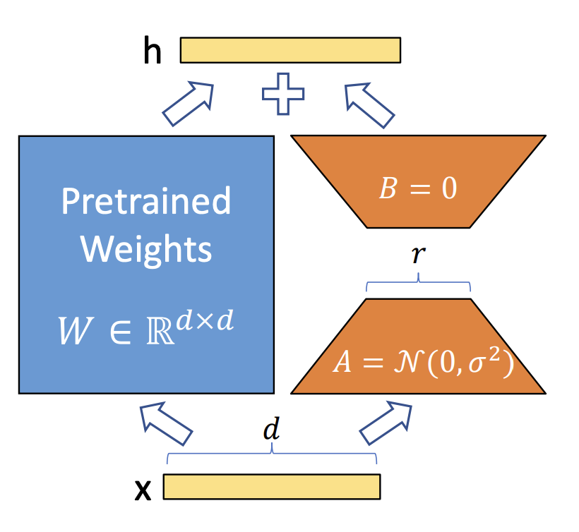
Specifically, for a weight matrix \(W \in \mathbb{R}^{d \times d}\), LoRA introduces two low-rank matrices \(A \in \mathbb{R}^{r \times d}\) and \(B \in \mathbb{R}^{d \times r}\), where \(r\) is the rank of the decomposition and is much smaller than \(d\). During fine-tuning, instead of updating the original weight matrix \(W\), we only update the low-rank matrices \(A\) and \(B\). The effective weight matrix during fine-tuning becomes:
\[ W'x = W_0x + \Delta Wx = Wx + BAx \tag{14}\]
where \(W_0\) is the original weight, \(\Delta W = BA\) represents the low-rank update to the original weight matrix. By choosing a small rank \(r \ll d\), we can significantly reduce the number of trainable parameters, making it feasible to fine-tune large models like PaliGemma on limited hardware. And LoRa can be applied to any linear layers in the model, including the attention (q, k, v, projection) and feed-forward layers in both the vision encoder and language model. During the fine-tuning process, there is also a \(\alpha\) parameter that scales the LoRA update to control its impact on the original weights by adjusting the learning dynamics. The scaled update becomes:
\[ W'x = Wx + \frac{\alpha}{r} BAx \tag{15}\]
We can build a LoRA module that can be easily integrated into existing linear layers in the PaliGemma model. Here is a simple implementation of the LoRA module:
class LoraLinear(nn.Linear):
    def __init__(
        self,
        in_features,
        out_features,
        bias=True,
        r: int = 8,
        alpha: float = 16.0,
        dropout: float = 0.0,
        std: float = 0.01,
    ):
        super().__init__(in_features, out_features, bias=bias)
        assert r > 0, "LoRA rank r must be > 0"
        self.r = r
        self.std = std
        self.alpha = float(alpha)
        self.scaling = self.alpha / r
        self.lora_enabled = True
        self.lora_dropout = nn.Dropout(dropout) if dropout and dropout > 0 else nn.Identity()

        # freeze base
        # This will be copy by-copy in the `get_lora_model` function, so it's safe to do this in-place here.
        self.weight.requires_grad_(False)
        if self.bias is not None:
            self.bias.requires_grad_(False)

        # LoRA params
        self.lora_A = nn.Parameter(torch.empty(r, in_features))
        self.lora_B = nn.Parameter(torch.empty(out_features, r))
        self.reset_lora_parameters()

        # track merge state
        self._merged = False

    def forward(self, x: torch.Tensor) -> torch.Tensor:
        out = F.linear(x, self.weight, self.bias)
        if self.lora_enabled and not self._merged:
            # h = F.linear(self.lora_dropout(x), self.lora_A)  # [*, r]
            # out = out + F.linear(h, self.lora_B) * self.scaling
            x = self.lora_dropout(x)
            h = x @ self.lora_A.T  # [*, r]
            h = h @ self.lora_B.T  # [*, out]
            h = h * self.scaling
            out = out + h

        return out
In this implementation, the LoraLinear class extends the standard nn.Linear layer by adding two low-rank matrices lora_A and lora_B. The forward method computes the original linear transformation and adds the LoRA update if LoRA is enabled. The LoRA parameters are initialized using a specific initialization strategy to ensure effective training.
2.7.1 Initalization of LoRA Parameters
The LoRA parameters are initialized using a specific strategy to ensure effective training. The initialization is done as follows:
\[ \begin{split} \text{lora\_A} \sim \mathcal{N}(0, \sigma^2), \quad \sigma & = 0.01 \\ \text{lora\_B} & = 0 \end{split} \tag{16}\]
This initialization ensures that at beginning of the training, the LoRA weight has none impact \(\Delta W = BA = 0\) on the original weight matrix, allowing the model to start from its pre-trained state and gradually adapt through the low-rank updates during fine-tuning. Here is the implementation of the initialization in code: