Reinforcement Learning in LLM
In previous blogs, we discussed the fundamental concepts of large language models (LLMs), including their architecture and supervised training via next-token prediction. Through maximum likelihood training, we are able to build models that generate fluent text matching the distribution of the training data.However, this is only the starting point. Modern LLM systems, such as ChatGPT, do not merely imitate text from the data distribution. They are expected to generate responses that are helpful, truthful, harmless, and aligned with human preferences. Moreover, recent models such as DeepSeek-R1 (DeepSeek-AI et al. 2025) demonstrate advanced reasoning capabilities, including the explicit generation of intermediate reasoning steps before producing a final answer.How are such behaviors achieved? How can a model be trained to optimize objectives that go beyond next-token likelihood — objectives that involve sequence-level evaluation, preference alignment, and verifiable correctness? The key lies in Reinforcement Learning (RL).
In this blog, we explore how reinforcement learning is used to post-train large language models to improve their performance, robustness, reasoning ability, and alignment with human values. We begin by formulating the LLM generation process as an RL problem, defining states, actions, policies, and rewards in the context of language modeling. We then introduce widely adopted reinforcement learning from human preference methods (RLHF), focusing on algorithms such as Proximal Policy Optimization (PPO)(Ouyang et al. 2022) and Direct Preference Optimization (DPO)(Rafailov et al. 2024). Next, we discuss Reinforcement Learning with Verifiable Rewards (RLVR) and representative approaches including GRPO(Shao et al. 2024), GSPO(Zheng et al. 2025), DAPO(Yu et al. 2025), SAPO(Gao et al. 2025), and the state-of-the-art GDPO(Liu et al. 2026). We also survey practical training frameworks for LLM-RL, such as Verl, Open-RLHF and so on.
Finally, we conclude with key challenges, open problems, and emerging research directions in applying reinforcement learning to large language models.
But before we dive into the specific algorithms and techniques, let’s first review some fundamental concepts and notations in reinforcement learning that will be essential for understanding the subsequent discussions.
1 Preliminaries
In this section, we will review some fundamental concepts and notations that are essential for understanding reinforcement learning (RL) and its application in large language models (LLMs). We will cover key topics such as entropy, KL-Divergence, Monte Carlo estimation and importance sampling. These concepts will provide a solid foundation for the subsequent discussions on RL algorithms and their integration with LLMs. For readers who are already familiar with these topics, feel free to skip this section and proceed to the next part of the blog.
1.1 Entropy
Entropy is a measure of uncertainty or randomness in a probability distribution. In the context of reinforcement learning, entropy is often used to encourage exploration by promoting diverse action selection. The entropy of a discrete probability distribution \(p(x)\) is defined as:
\[ H(p) = - \sum_{x} p(x) \log p(x) \tag{1}\]
For continuous distributions, the entropy is defined as: \[ H(p) = - \int p(x) \log p(x) dx \tag{2}\]
One thing to note is that:
- Higher entropy indicates more uncertainty and exploration
- Lower entropy indicates more certainty and exploitation
For the discrete case, the entropy is maximized when the distribution is uniform \(p(x) = \frac{1}{|X|}\), i.e., all outcomes are equally likely. In contrast, the entropy is minimized (zero) when the distribution is deterministic, i.e., one outcome has probability 1 and all others have probability 0.
1.2 KL-Divergence
The Kullback-Leibler (KL) Divergence is a measure of how one probability distribution diverges from a second, expected probability distribution. In reinforcement learning, KL-Divergence is often used to quantify the difference between two policies, which is useful for policy optimization and regularization. The KL-Divergence from distribution \(P\) to distribution \(Q\) is defined as: \[ D_{KL}(P \| Q) = \sum_{x} P(x) \log \frac{P(x)}{Q(x)} \tag{3}\]
For continuous distributions, the KL-Divergence is defined as: \[ D_{KL}(P \| Q) = \int P(x) \log \frac{P(x)}{Q(x)} dx \tag{4}\]
The KL-Divergence has several important properties:
- Non-negativity: \(D_{KL}(P \| Q) \geq 0\), with equality if and only if \(P = Q\) almost everywhere.
- Asymmetry: \(D_{KL}(P \| Q) \neq D_{KL}(Q \| P)\) in general.
To compute the KL-Divergence between two distributions \(P\) and \(Q\) in practice, we can use the following function:
import torch.nn.functional as F

def compute_kl_divergence(P_logits: torch.Tensor, Q_logits: torch.Tensor) -> torch.Tensor:
    """
    P_logits (torch.Tensor): Logits of distribution P (shape: [batch_size, num_classes])
    Q_logits (torch.Tensor): Logits of distribution Q (shape: [batch_size, num_classes])
    """
    log_prob_p = F.log_softmax(P_logits, dim=-1)  # Log probabilities of P
    log_prob_q = F.log_softmax(Q_logits, dim=-1)  # Log probabilities of Q

    kl_divergence = torch.sum(torch.exp(log_prob_p) * (log_prob_p - log_prob_q), dim=-1)  # KL Divergence
    return kl_divergence
NOTE Further Reading about Entropy & KL Divergence
For those who want to dive deeper into Entropy and KL-Divergence, I highly recommend to check out my previous blog: From Entropy to KL Divergence: A Comprehensive Guide
1.3 Monte Carlo Estimation
In the practice of machine learning and reinforcement learning, we often encounter situations where we need to compute expectations of functions with respect to complex probability distributions. Monte Carlo estimation is a powerful technique that allows us to approximate these expectations using random sampling. The basic idea is:
draw samples from the target distribution and use them to compute an empirical average of the function of interest.
Due to the law of large numbers, this empirical average converges to the true expectation as the number of samples increases.
For example, suppose we want to estimate the expectation of a function \(f(x)\) with respect to a probability distribution \(p(x)\): \[ \begin{split} \mathbb{E}_{x \sim p(x)}[f(x)] & = \int f(x) p(x) dx \\ & \approx \frac{1}{N} \sum_{i=1}^{N} f(x^{(i)}) \quad \text{where } x^{(i)} \sim p(x) \end{split} \tag{5}\]
This is the foundation of many algorithms in reinforcement learning, where we need to estimate expected returns, value functions, and policy gradients based on sampled trajectories.
For the KL-Divergence between two distributions \(P\) and \(Q\), we can use Monte Carlo estimation to approximate it as follows: \[ D_{KL}(P || Q) = \mathbb{E}_{x \sim P} \left[ \log \frac{P(x)}{Q(x)} \right] \approx \frac{1}{N} \sum_{i=1}^{N} \log \frac{P(x^{(i)})}{Q(x^{(i)})} \quad \text{where } x^{(i)} \sim P(x) \tag{6}\]
1.4 Importance Sampling
When we want to estimate an expectation with respect to a target distribution \(p(x)\), but we can only sample from a different distribution \(q(x)\) (known as the proposal distribution), we can use importance sampling to correct for the discrepancy between the two distributions. The key idea is to reweight the samples drawn from the proposal distribution by the ratio of the target and proposal densities. The expectation of a function \(f(x)\) with respect to the target distribution \(p(x)\) can be expressed as:
\[ \mathbb{E}_{x \sim p(x)}[f(x)] = \int f(x) p(x) dx = \int f(x) \frac{p(x)}{\textcolor{red}{q(x)}} \textcolor{red}{q(x)} dx = \mathbb{E}_{x \sim \textcolor{red}{q(x)}}\left[ f(x) \frac{p(x)}{\textcolor{red}{q(x)}} \right] \tag{7}\]
Using Monte Carlo estimation, we can approximate this expectation using samples drawn from the proposal distribution \(q(x)\): \[ \mathbb{E}_{x \sim p(x)}[f(x)] \approx \frac{1}{N} \sum_{i=1}^{N} f(x^{(i)}) \frac{p(x^{(i)})}{\textcolor{red}q(x^{(i)})} \quad \text{where } x^{(i)} \sim \textcolor{red}{q(x)} \tag{8}\]
where \(\frac{p(x^{(i)})}{q(x^{(i)})}\) is known as the importance weight / importance ratio. Importance sampling is particularly useful in reinforcement learning when we want to evaluate or improve a policy using data collected from a different policy.
2 Notations
There are various notations used in the literature of reinforcement learning (RL) and large language models (LLMs). To maintain consistency and clarity throughout this blog, we will define and use a standard set of notations as following:
| Notation | Meaning | Description |
|---|---|---|
| \(\pi_{\theta}\) | Policy | A mapping function from states to a probability distribution over actions. |
| \(s_t\) | State at time \(t\) | The current context or input to the LLM at time step \(t\). This could include the text generated so far and any other relevant information. |
| \(a_t\) | Action at time \(t\) | The token or word generated by the LLM at time step \(t\). |
| \(r_t\) | Reward at time \(t\) | A scalar value received after taking action \(a_t\) in state \(s_t\). It indicates the quality of the generated token in the context of the overall text generation task. |
| \(R_t\) | Return at time \(t\) | The cumulative reward received from time step \(t\) onwards. It is often used to evaluate the long-term effectiveness of the policy. |
| \(\gamma\) | Discount factor | A value between 0 and 1 that determines the importance of future rewards. A higher value places more emphasis on future rewards. |
| \(V^{\pi}(s)\) | Value function / State-value function | The expected return when starting from state \(s\) and following policy \(\pi\). It measures the long-term value of being in state \(s\). |
| \(Q^{\pi}(s, a)\) | Action-value function | The expected return when starting from state \(s\), taking action \(a\), and thereafter following policy \(\pi\). It evaluates the quality of taking action \(a\) in state \(s\). |
| \(A^{\pi}(s, a)\) | Advantage function | The difference between the action-value function and the value function: \(A^{\pi}(s, a) = Q^{\pi}(s, a) - V^{\pi}(s)\). It indicates how much better or worse taking action \(a\) in state \(s\) is compared to the average action. |
| \(H(p)\) | Entropy of distribution \(p\) | A measure of uncertainty or randomness in the policy’s action selection. Higher entropy indicates more exploration. |
| \(\tau\) | Trajectory / Episode / Rollout | A sequence of states, actions, and rewards generated by following a policy from an initial state to a terminal state. Can be viewd as a sequence of state and action pairs: \(\tau = (s_0, a_0, s_1, a_1, ..., s_T, a_T)\) |
| \(\rho(\tau)\) | Importance Sampling Ratio | The ratio of probabilities of a trajectory under two different policies: \(\frac{\pi_{\theta}(\tau)}{\pi_{\theta_{old}}(\tau)}\) |
3 Review of Reinforcement Learning
In this section, we will provide a brief overview of key reinforcement learning (RL) concepts that are relevant to understanding how RL is applied in large language models (LLMs). We will cover the fundamental components of RL, including the agent, environment, states, actions, rewards, and policies. Additionally, we will discuss common RL algorithms and techniques that are often employed in the context of LLMs.
TIP: Dig into Reinforcement Learning
For those who what to dig deeper into RL, I highly recommend the following resources:
- Reinforcement learning: An introduction: A comprehensive textbook by Sutton and Barto that covers the fundamentals of RL.
- Stanford CS234 Reinforcement Learning: This course provides lectures and video materials on various RL topics, it can be seen as complementary to the Sutton and Barto book.
- UCB CS285 Deep Reinforcement Learning: This course focuses on deep reinforcement learning techniques and their applications. (The first several lectures cover basic Deep RL concepts and Policy Gradient methods, the review section in this blog is heavily inspired by these lectures)
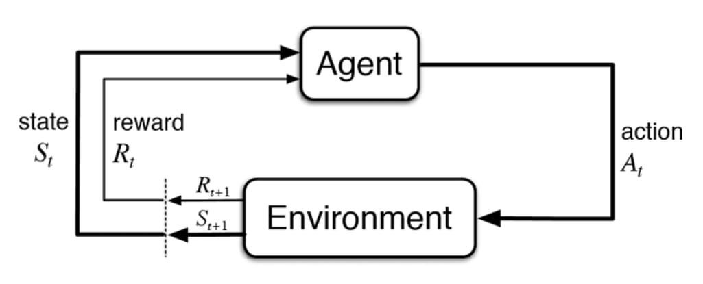
Reinforcement Learning (RL) is a framework for learning to make sequential decisions by interacting with an environment. In RL, an agent learns to take actions in an environment in order to maximize cumulative rewards over time. The key components of RL include:
- Agent: The learner or decision-maker that interacts with the environment.
- Environment: The external system with which the agent interacts. It provides feedback in the form of rewards and new states based on the agent’s actions.
- State (\(s_t\)): A representation of the current situation or context at time step \(t\).
- Action (\(a_t\)): A decision or move made by the agent at time step \(t\).
- Reward (\(r_t\)): A scalar feedback signal received after taking action \(a_t\) in state \(s_t\). It indicates the immediate value of the action taken.
- Policy (\(\pi\)): A mapping from states to a probability distribution over actions. It defines the agent’s behavior and decision-making strategy.
We can see how those components related in the following figure:
The goal of reinforcement learning is to find an optimal policy \(\pi^*\) that maximizes the expected cumulative reward (return) over time. Let’s first define the objective function \(J(\pi)\) that we want to maximize:
\[ J(\pi) = \mathbb{E}_{\tau \sim \pi} \left[\sum_{t=0}^{T} r_t \right] \tag{9}\]
where:
- \(\tau\) represents a trajectory (sequence of states, actions) generated by following policy \(\pi\).
Let’s expand the trajectory expectation:
\[ p(\tau | \pi) = p(s_0) \prod_{t=0}^{T} \pi(a_t | s_t) p(s_{t+1} | s_t, a_t) \tag{10}\]
Where:
- \(p(s_0)\) is the initial state distribution, which is often given by the environment or can be assumed to be a fixed distribution.
- \(\pi(a_t | s_t)\) is the policy’s probability of taking action \(a_t\) in state \(s_t\), this is the part we can control and optimize in policy gradient methods.
- \(p(s_{t+1} | s_t, a_t)\) is the environment’s transition probability from state \(s_t\) to \(s_{t+1}\) given action \(a_t\). We usually do not have access to this transition probability in model-free RL.
We know that the policy \(\pi_{\theta}\) is parameterized by \(\theta\) (e.g., neural network weights). The goal of RL is to optimize the policy parameters \(\theta\) to maximize the expected return \(J(\pi_{\theta})\). This is typically done using gradient-based optimization methods, where we compute the gradient of the objective function with respect to the policy parameters:
\[ \nabla_{\theta} J(\pi_{\theta}) = \nabla_{\theta} \mathbb{E}_{\tau \sim \pi_{\theta}} \left[\sum_{t=0}^{T} r_t \right] \tag{11}\]
However, we cannot get the gradient directly because:
- The expectation is over trajectories \(\tau\), which depend on the policy \(\pi_{\theta}\).
- The environment dynamics (transition probabilities) are usually unknown.
To address this, we can use the Log-Derivative Trick (also known as the Score Function Estimator) to rewrite the gradient:
\[ \nabla_{\theta} P_{\theta}(x) = P_{\theta}(x) \nabla_{\theta} \log P_{\theta}(x) \tag{12}\]
Applying Equation 12 to our policy gradient, we have:
\[ \begin{split} \nabla_{\theta} J(\pi_{\theta}) & = \int \nabla_{\theta} p(\tau | \pi_{\theta}) \sum_{t=0}^{T} r_t d\tau \\ & = \mathbb{E}_{\tau \sim \pi_{\theta}} \left[ \nabla_{\theta} \log \pi_{\theta}(\tau) \sum_{t=0}^{T} r_t \right] \end{split} \tag{13}\]
Where:
- \(\log \pi_{\theta}(\tau)\) is the log-probability of the trajectory \(\tau\) under the policy \(\pi_{\theta}\).
- \(\sum_{t=0}^{T} r_t\) is the cumulative reward for the trajectory.
Plugging in the trajectory probability from Equation Equation 10, we can further expand the policy gradient:
\[ \nabla_{\theta} J(\pi_{\theta}) = \mathbb{E}_{\tau \sim \pi_{\theta}} \left[ \left( \sum_{t=0}^{T} \nabla_{\theta} \log \pi_{\theta}(a_t | s_t) \right) \left( \sum_{t=0}^{T} r_t \right) \right] \tag{14}\]
where \(\sum_{t=0}^{T} \nabla_{\theta} \log \pi_{\theta}(a_t | s_t)\) is the sum of log-probability gradients of the actions taken along the trajectory, since the transition probabilities \(p(s_{t+1} | s_t, a_t)\) do not depend on \(\theta\), they do not contribute to the gradient.
To get this expectation, we can use Monte Carlo estimation (Section 1.3) by sampling trajectories from the current policy \(\pi_{\theta}\) and computing the empirical average:
\[ \nabla_{\theta} J(\pi_{\theta}) \approx \frac{1}{N} \sum_{i=1}^{N} \left[ \left( \sum_{t=0}^{T} \textcolor{cyan}{\nabla_{\theta} \log \pi_{\theta}(a_t^{(i)} | s_t^{(i)})} \right) \left( \sum_{t=0}^{T} r_t^{(i)} \right) \right] \tag{15}\]
WAIT!! This look familiaer? Yes, in the Deep Learning 101. We know the classification loss gradient can be written as: \[ \begin{split} \nabla_{\theta} \mathcal{L}_{\text{classification}} & = - \mathbb{E}_{(x, y) \sim \mathcal{D}} \left[ \nabla_{\theta} \log p_{\theta}(y | x) \right] \\ & \approx - \frac{1}{N} \sum_{i=1}^{N} \textcolor{cyan}{\nabla_{\theta} \log p_{\theta}(y^{(i)} | x^{(i)})} \end{split} \tag{16}\]
Where \(p_{\theta}(y|x)\) is the model’s predicted probability for label \(y\) given input \(x\).
The similarity between Equation (Equation 15) and Equation (Equation 16) highlights that both RL policy gradients and supervised learning gradients can be computed using
This form the most foundation of policy gradient methods in RL, the algorithms to optimize the policy parameters \(\theta\) by is called REINFORCE algorithm.
However, the basic REINFORCE algorithms suffers from several issues, one of the major issue is the high variance of the gradient estimates, which can lead to unstable and slow learning. To address this, several variance reduction techniques have been developed, such as using baselines (e.g., value functions) to reduce variance without introducing bias.
\[ \nabla_{\theta} J(\pi_{\theta}) \approx \frac{1}{N} \sum_{i=1}^{N} \left[ \left( \sum_{t=0}^{T} \nabla_{\theta} \log \pi_{\theta}(a_t^{(i)} | s_t^{(i)}) \right) \left( \sum_{t=0}^{T} r_t^{(i)} - b(s_t^{(i)}) \right) \right] \tag{17}\]
Question: Why this is Unbiased?
The baseline \(b(s_t)\) does not depend on the action \(a_t\), so it does not introduce bias into the gradient estimate. When we take the expectation over the trajectories, the term involving the baseline cancels out because:
\[ \mathbb{E}_{\tau \sim \pi_{\theta}} \left[ \nabla_{\theta} \log \pi_{\theta}(a_t | s_t) b(s_t) \right] = b(s_t) \mathbb{E}_{\tau \sim \pi_{\theta}} \left[ \nabla_{\theta} \log \pi_{\theta}(a_t | s_t) \right] = 0 \]
We are safe to subtract any baseline without introducing bias as long as it does not depend on the action \(a_t\). A common choice for the baseline is the value function \(V^{\pi}(s_t)\), which estimates the expected return from state \(s_t\) under policy \(\pi\). Using the value function as a baseline helps to reduce variance by centering the rewards around their expected values.
\[ \nabla_{\theta} J(\pi_{\theta}) \approx \frac{1}{N} \sum_{i=1}^{N} \left[ \left( \sum_{t=0}^{T} \nabla_{\theta} \log \pi_{\theta}(a_t^{(i)} | s_t^{(i)}) \right) \left( \sum_{t=0}^{T} r_t^{(i)} - V^{\pi}(s_t^{(i)}) \right) \right] \tag{18}\]
The other thing to can use to reduce variance is by applying causality, which means that an action at time step \(t\) can only affect future rewards, not past rewards. Therefore, we can rewrite the policy gradient to only consider future rewards from time step \(t\) onwards:
\[ \nabla_{\theta} J(\pi_{\theta}) \approx \frac{1}{N} \sum_{i=1}^{N} \left[ \sum_{t=0}^{T} \nabla_{\theta} \log \pi_{\theta}(a_t^{(i)} | s_t^{(i)}) \left( \sum_{t'=t}^{T} r_{t'}^{(i)} - V^{\pi}(s_t^{(i)}) \right) \right] \tag{19}\]
Here, we give \(\sum_{t'=t}^{T} r_{t'}\) a special name called reward to go(also known as return) \(R_t\):
\[ R_t = \sum_{t'=t}^{T} r_{t'} \tag{20}\]
Take a close look at reward to go \(R_t\), we can see that it is an estimate of expected reward if we take action \(a_t\) at state \(s_t\) and follow policy \(\pi\) thereafter. This is exactly the definition of action-value function \(Q^{\pi}(s_t, a_t)\):
\[ Q^{\pi}(s_t, a_t) = \mathbb{E}_{\tau \sim \pi} \left[ R_t | s_t, a_t \right] \tag{21}\]
So, we can further rewrite the policy gradient as:
\[ \nabla_{\theta} J(\pi_{\theta}) \approx \frac{1}{N} \sum_{i=1}^{N} \left[ \sum_{t=0}^{T} \nabla_{\theta} \log \pi_{\theta}(a_t^{(i)} | s_t^{(i)}) \left( Q^{\pi}(s_t^{(i)}, a_t^{(i)}) - V^{\pi}(s_t^{(i)}) \right) \right] \tag{22}\]
Where the term in the parentheses is known as the advantage function \(A^{\pi}(s_t, a_t)\): \[ A^{\pi}(s_t, a_t) = Q^{\pi}(s_t, a_t) - V^{\pi}(s_t) \tag{23}\]
And we know the action-value function \(Q^{\pi}(s_t, a_t)\) and value function \(V^{\pi}(s_t)\) can be estimated using various methods, such as Monte Carlo estimation, Temporal Difference (TD) learning, or function approximation (e.g., neural networks), according to the Ballman equation, the value function and action-value function satisfy the following relationships:
\[ V^{\pi}(s_t) = \mathbb{E}_{a_t \sim \pi} \left[ Q^{\pi}(s_t, a_t) \right] \tag{24}\]
And \[ Q^{\pi}(s_t, a_t) = \mathbb{E}_{s_{t+1} \sim p} \left[ r_t + \gamma V^{\pi}(s_{t+1}) \right] \tag{25}\]
So, to train an RL agent using policy gradient methods, we typically follow these steps:
- Collect Trajectories: Sample trajectories by executing the current policy \(\pi_{\theta}\) in the environment.
- Estimate Returns: Compute the returns \(R_t\) for each time step in the collected trajectories.
- Estimate Value Functions: Estimate the value function \(V^{\pi}(s_t)\) and action-value function \(Q^{\pi}(s_t, a_t)\) using the collected data.
- Compute Policy Gradient: Use the estimated value functions to compute the policy gradient using Equation {#eq-policy-gradient-with-advantage}.
- Update Policy Parameters: Update the policy parameters \(\theta\) using gradient ascent: \[ \theta \leftarrow \theta + \alpha \nabla_{\theta} J(\pi_{\theta}) \] Where \(\alpha\) is the learning rate.
This is known as Actor-Critic method, where the policy (actor) is updated using value function estimates (critic) to reduce variance and improve learning stability.
3.1 On Policy vs Off Policy
So far, we have discussed policy gradient methods in the context of on-policy learning, where the policy used to collect data (trajectories) is the same as the policy being optimized. However, there are also off-policy methods, where the data is collected using a different policy (behavior policy) than the one being optimized (target policy). The goal of off-policy methods is to leverage data collected from various policies to improve learning efficiency and stability. The main idea behind off-policy learning is to use importance sampling (Section 1.4) to correct for the distribution mismatch between the behavior policy and the target policy.
Let’s re-write the policy gradient using importance sampling, what we have is the state action reward pairs collected from the old policy \(\pi_{\theta_{old}}\), but we want to optimize the new policy \(\pi_{\theta}\):
\[ \begin{split} \nabla_{\theta} J(\pi_{\theta}) & = \mathbb{E}_{\tau \sim \pi_{\theta}} \left[ \nabla_{\theta} \log \pi_{\theta}(\tau) \sum_{t=0}^{T} r_t \right] \\ & = \mathbb{E}_{\tau \sim \pi_{\theta_{old}}} \left[ \underbrace{\frac{\pi_{\theta}(\tau)}{\pi_{\theta_{old}}(\tau)}}_{\text{Importance Ratio}} \nabla_{\theta} \log \pi_{\theta}(\tau) \sum_{t=0}^{T} r_t \right] \end{split} \tag{26}\]
Let’s expand the importance ratio: \[ \frac{\pi_{\theta}(\tau)}{\pi_{\theta_{old}}(\tau)} = \prod_{t=0}^{T} \frac{\pi_{\theta}(a_t | s_t)}{\pi_{\theta_{old}}(a_t | s_t)} \tag{27}\]
Plugging this back to Equation 26, we have: \[ \begin{split} \nabla_{\theta} J(\pi_{\theta}) &= \mathbb{E}_{\tau \sim \pi_{\theta_{old}}} \left[ \left( \prod_{t=0}^{T} \frac{\pi_{\theta}(a_t | s_t)}{\pi_{\theta_{old}}(a_t | s_t)} \right) \left( \nabla_{\theta} \log \pi_{\theta}(\tau) \sum_{t=0}^{T} r_t \right) \right] \\ & \approx \frac{1}{N} \sum_{i=1}^{N} \left[ \left( \prod_{t=0}^{T} \frac{\pi_{\theta}(a_t^{(i)} | s_t^{(i)})}{\pi_{\theta_{old}}(a_t^{(i)} | s_t^{(i)})} \right) \left( \sum_{t=0}^{T} \nabla_{\theta} \log \pi_{\theta}(a_t^{(i)} | s_t^{(i)}) \right) A^{(i)} \right] \end{split} \tag{28}\]
There are several challenges with off-policy policy gradient methods:
As we can see, this algorithm Algorithm 1 to more
4 Mapping LLM Post Training as RL Problems
In the previous section, we have reviewed the fundamental concepts of reinforcement learning (RL) and policy gradient methods. Now, we will explore how these RL concepts can be applied to large language models (LLMs) in the context of post-training fine-tuning. We will discuss how to formulate the LLM fine-tuning process as an RL problem, including defining states, actions, rewards, and policies. This mapping will provide a foundation for understanding various RL algorithms used in LLMs, such as Reinforcement Learning from Human Feedback (RLHF) and Reinforcement Learning from Verified Rewards (RLVR).
4.1 State, Action, Policy in LLM
In the context of large language models (LLMs), we can map the components of reinforcement learning (RL) to the LLM fine-tuning process as follows:
- State (\(s_t\)): The state at time step \(t\) can be defined as the current context or input to the LLM. This includes the text generated so far, any preceding prompts, and potentially other relevant information such as metadata or user preferences. The state encapsulates all the information that the model has access to when generating the next token.
- Action (\(a_t\)): The action at time step \(t\) corresponds to the token or word generated by the LLM. The action space is typically the vocabulary of the language model, and the model selects an action based on its current policy (i.e., the probability distribution over the vocabulary given the current state).
- Policy (\(\pi_{\theta}\)): The policy in the context of LLMs is represented by the language model itself, parameterized by \(\theta\). The policy defines the probability distribution over actions (tokens) given the current state (context). The policy can be expressed as \(\pi_{\theta}(a_t | s_t)\), which gives the probability of generating token \(a_t\) given the context \(s_t\).
- Reward (\(r_t\)): The reward at time step \(t\) is a scalar value that indicates the quality of the generated token in the context of the overall text generation task. Rewards can be derived from various sources, such as human feedback, automated evaluation metrics, or other criteria that reflect the desired behavior of the LLM. The reward signal guides the learning process by providing feedback on the effectiveness of the generated tokens.
One thing good about LLM is that
Because of this, we can focus on optimizing the policy (the LLM) directly based on the reward signals without worrying about modeling the environment transitions.
For example, at the begin of training, we have text(prompt) like: “The capital of France is”, this is our initial state \(s_0\).
- \(s_0\) = “The capital of France is”
- \(a_0 \sim \text{softmax}(f_{\theta}(s_0))\) = ” Paris”
- \(s_1 = (s_0, a_0)\) = “The capital of France is Paris”
- \(a_1 \sim \text{softmax}(f_{\theta}(s_1))\) = “.”
- \(s_2 = (s_1, a_1)\) = “The capital of France is Paris.”
- …
This process continues until the model generates a complete response or reaches a predefined stopping criterion, when the <eos> token is generated or the max length is reached. In the end, we got trajectory/episode/rollout \(\tau = (s_0, a_0, s_1, a_1, ..., s_T, a_T)\).
4.2 Reward Design Challenges in LLM
In reinforcement learning for large language models (LLMs), the reward function plays a crucial role in guiding the model’s learning process. The reward function defines the objectives and desired behaviors that the LLM should exhibit during text generation. However, designing effective reward functions for LLMs can be challenging:
- Sparse Rewards: In many cases, rewards may only be provided at the end of a generated sequence, making it difficult to attribute credit to individual token (action) generations.
- Ambiguous Objectives: The desired behavior of LLMs can be complex and multifaceted, making it hard to define a single reward function that captures all aspects of quality.
- Human Feedback: When using human feedback as a reward signal, it can be noisy, inconsistent, and expensive to obtain.
- Scalability: As LLMs generate long sequences, computing rewards for every token can be computationally expensive.
- Exploration vs. Exploitation: Balancing the need for exploration (trying new token generations) and exploitation (generating high-reward tokens) is crucial for effective learning.
In the following sections, we will explore specific RL algorithms that have been applied to LLM fine-tuning, including Reinforcement Learning from Human Feedback (RLHF) and Reinforcement Learning from Verified Rewards (RLVR). We will discuss how these algorithms leverage the RL framework to improve the performance and alignment of LLMs with human preferences
5 Reinforcement Learning from Human Feedback(RLHF)
After Pre-Training and Supervised Fine-Tuning, Large Language Models(LLMs) can generate high-quality text, but they may not always align with human preferences or ethical guidelines. To address this, Reinforcement Learning from Human Feedback (RLHF) has emerged as a powerful technique to fine-tune LLMs using feedback from human evaluators. RLHF leverages reinforcement learning (RL) principles to optimize the LLM’s behavior based on human-provided rewards, guiding the model to generate text that better aligns with human values and expectations. (Ouyang et al. 2022)
Before diving into the RLHF algorithms, let’s first take a look at the data collection process for human feedback. The human feedback data is typically collected through the following steps:
- Prompt Generation: A set of prompts is created to elicit responses from the LLM. These prompts can be designed to cover a wide range of topics and scenarios to ensure diverse feedback.
- Model Response Generation: The LLM generates responses to the prompts, which are then presented to human evaluators for review.
- Human Evaluation: Human evaluators assess the generated responses based on various criteria, such as relevance, coherence, informativeness, and alignment with human values. They may provide feedback in the form of ratings, rankings, or qualitative comments.
- Reward Model Training: The collected human feedback is used to train a reward model that can predict the quality of generated responses based on the human evaluations. This reward model serves as a proxy for human preferences and is used to guide the reinforcement learning process in fine-tuning the LLM.
- Reinforcement Learning Fine-Tuning: The LLM is fine-tuned using reinforcement learning algorithms, such as Proximal Policy Optimization (PPO), to optimize the policy (the LLM) to maximize the expected reward as predicted by the reward model.
Here we will focus on the reinforcement learning fine-tuning step, specifically the PPO algorithm, which is commonly used in RLHF for LLMs. Assume we have already collected human feedback and trained a reward model \(R_{\phi}(s, a)\), we can now use PPO to fine-tune the LLM based on the learned reward model.
5.1 PPO
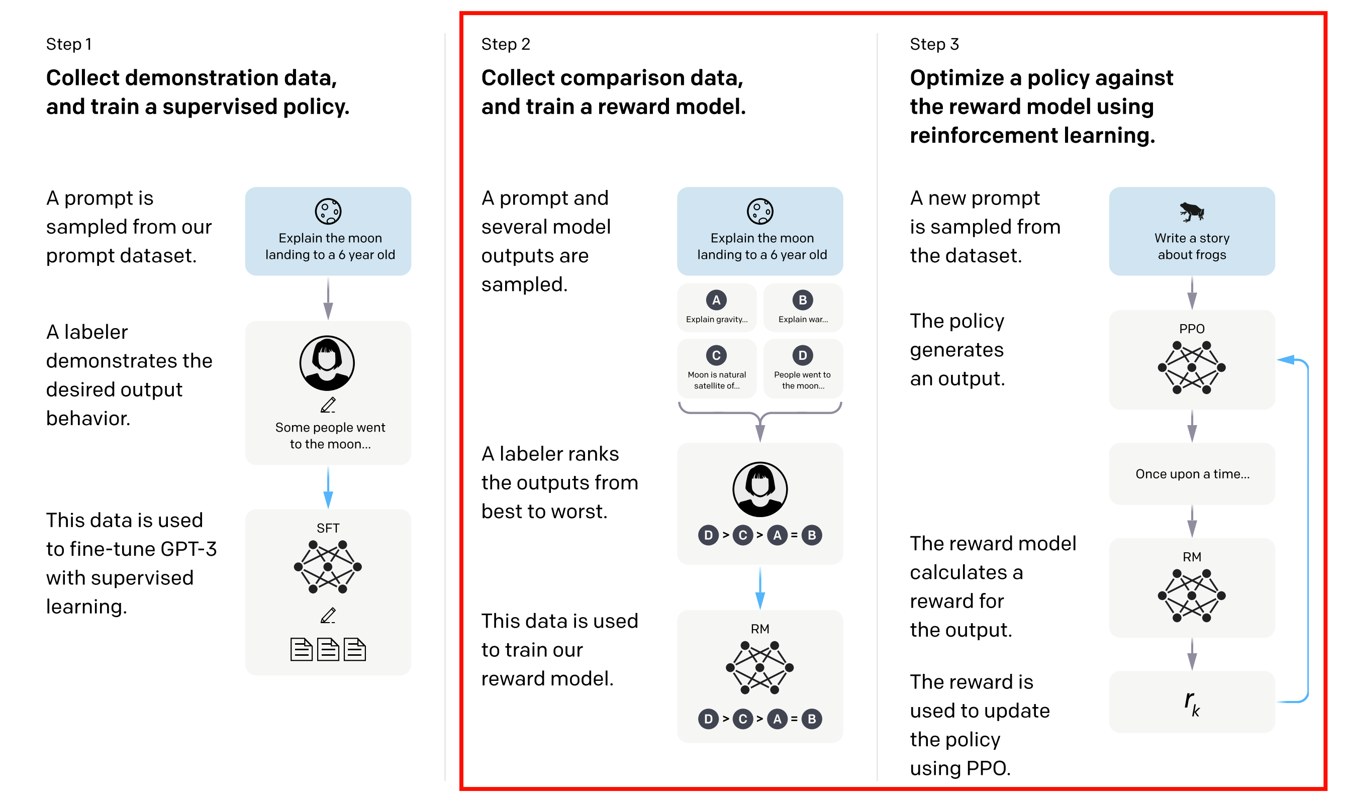
Following the foundational work of InstructGPT (Ouyang et al. 2022), Proximal Policy Optimization (PPO)(Schulman et al. 2017) has become one of the most widely used algorithms for implementing RLHF in large language models. We can see the PPO algorithm in the Figure 2. It has several steps:
- Collecting Human Feedback: Initially, the LLM generates responses to a set of prompts. Human evaluators then review these responses and provide feedback, typically in the form of rankings or ratings. This feedback serves as the basis for training a reward model.
- Training a Reward Model: A separate reward model is trained to predict the human feedback based on the generated responses. This model learns to assign higher scores to responses that align better with human preferences
- Fine-Tuning with PPO: The LLM is then fine-tuned using the PPO algorithm, which optimizes the policy (the LLM) to maximize the expected reward as predicted by the reward model. PPO uses a clipped objective function to ensure that policy updates are not too large, maintaining stability during training.
Here we just focus on the step 3, the PPO fine-tuning process. The PPO algorithm can be summarized as follows:
Let’s break down the PPO algorithm for RLHF in LLMs: 1. Initialization: We start with an initial policy \(\pi_{\theta_{old}}\), which can be a pre-trained language model or a supervised fine-tuned model. We also have a reward model \(R_{\phi}\) trained on human feedback, a reference policy \(\pi_{\text{ref}}\) (often the same as the initial policy), and a value function (critic) \(V_{\psi}\). We set the clipping parameter \(\epsilon\), KL coefficient \(\beta\), discount factor \(\gamma\), GAE parameter \(\lambda\), number of PPO epochs \(K\), minibatch size \(m\), and learning rates for policy and value updates. 2. Data Collection: We sample a batch of prompts and roll out the current policy \(\pi_{\theta_{old}}\) to generate responses. We compute the log-probabilities of the generated tokens under both the old policy and the reference policy, as well as the sequence-level reward from the reward model. 3. Reward Definition: We define per-timestep rewards that include a KL penalty based on the difference between the old policy and the reference policy, as well as a terminal reward from the reward model at the last token. 4. Advantage Estimation: We compute the advantages using Generalized Advantage Estimation (GAE) with the value function \(V_{\psi}\). 5. Policy and Value Optimization: We perform multiple epochs of optimization over shuffled minibatches. For each minibatch, we compute the PPO clipped objective for the policy and the value loss for the critic, and update the parameters accordingly. 6. Policy Synchronization: After the updates, we sync the old policy parameters with the new policy for the next rollout.
To apply this in code:
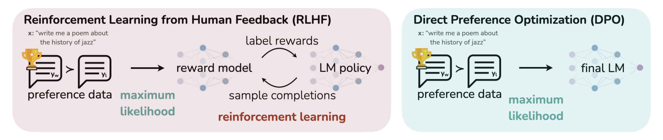
5.2 DPO
Direct Preference Optimization (DPO) (Rafailov et al. 2024) is a novel approach for fine-tuning large language models using human feedback without the need for a separate reward model.
5.3 REINFORCE Leave One-Out (RLOO)
Rein
5.4 ReMax
5.5 REINFORCE++
6 Reinforcement Learning from Verified Rewards(RLVR)
6.1 GRPO
6.1.1 Objective Function
The objective function of GRPO is defined as:
\[ \begin{split} \mathcal{J}_{\text{GRPO}}(\pi_\theta) &= \mathbb{E}_{q \sim \mathcal{D}} \;\mathbb{E}_{o \sim \pi_{\theta_{\text{old}}}(\cdot\mid q)} \left[ \sum_{t=1}^{|o|} \min \Big( \rho_t \hat{A}_{t}, \text{clip}\big( \rho_t, 1 - \epsilon_{\text{clip}}, 1 + \epsilon_{\text{clip}} \big)\hat{A}_{t} \Big) \;-\;\beta \,\text{KL}\big(\pi_\theta \,\|\, \pi_{\text{ref}}\big) \right] \\ &\approx \frac{1}{B}\sum_{b=1}^{B} \left[ \frac{1}{G}\sum_{i=1}^{G} \frac{1}{|o_{b,i}|}\sum_{t=1}^{|o_{b,i}|} \min \Big( \rho_{b,i,t} \hat{A}_{b,i,t}, \text{clip}\big( \rho_{b,i,t}, 1 - \epsilon_{\text{clip}}, 1 + \epsilon_{\text{clip}} \big)\hat{A}_{b,i,t} \Big) \;-\;\beta \,\text{KL}\big(\pi_\theta \,\|\, \pi_{\text{ref}}\big) \right] \end{split} \tag{29}\]
Where:
\[ \mathcal{J}_{\text{GRPO}}(\pi_\theta) = \tag{30}\]
其中:
\[ \rho(o_{i,t}) = \frac{\pi_\theta(o_{i,t}|q, o_{i,<t})}{\pi_{\text{ref}}(o_{i,t}|q, o_{i,<t})} \tag{31}\]
6.2 Dr.GRPO
6.3 DAPO
6.4 GSPO
6.5 CISPO
6.6 SAPO
6.7 GDPO
7 LLM-RL in Practice
7.1 TRL: Transformer Reinforcement Learning
7.2 verl: Volcano Engine Reinforcement Learning for LLMs
7.3 OpenRLHF
7.4 SWIFT (Scalable lightWeight Infrastructure for Fine-Tuning)
This is the test of Code-Block 1
8 Multi-Turn RL in LLMs
So far, we have discussed RL algorithms for fine-tuning LLMs in a single-turn setting, where the model generates a response based on a given prompt. However, in many real-world applications, LLMs are used in multi-turn interactions, such as chatbots or dialogue systems, where the model needs to generate responses over multiple turns of conversation. This means we have \(\text{history}_t, s_t, \text{think}_t, a_t\) at each time step \(t\), where \(\text{history}_t\) is the conversation history up to time \(t\), defined as \(\text{history}_t = s_0, \text{think}_0, a_0, s_1, \text{think}_1, a_1, ..., s_{t-1}, \text{think}_{t-1}, a_{t-1}, s_t\). The model needs to generate a response \(a_t\) based on the current state \(s_t\) and the conversation history \(\text{history}_t\).
9 Challenges & Further Direction
10 Summary
11 Appendix
11.1 Code Snippets
In this section, we provide some code snippets to illustrate the implementation of key components in reinforcement learning for large language models (LLMs). These snippets are meant to serve as examples and may not be complete or directly runnable without additional context and dependencies.
def get_log_probs(model, inputs, actions):
    """
    Compute log-probabilities of the actions given the inputs using the model.

    Args:
        model: The language model (e.g., a transformer) that outputs logits.
        inputs: The input sequences (contexts) for which to compute log-probs.
        actions: The token actions for which to compute log-probs.

    Returns:
        log_probs: A tensor of log-probabilities corresponding to the actions.
    """
    # Get logits from the model
    logits = model(inputs)  # Shape: [batch_size, seq_len, vocab_size]

    log_probs = torch.log_softmax(logits, dim=-1)  # Convert logits to log-probabilities

    # Gather log-probs for the taken actions
    log_probs = log_probs.gather(dim=-1, index=actions.unsqueeze(-1)).squeeze(-1)  # Shape: [batch_size, seq_len]

    return log_probs