02: An Image is Worth \(16 \times 16\) Words: Transformers for Image Recognition at Scale (Vision-Transformer )
Patch Embedding、Position Embedding、[CLS] Token 以及 Transformer 编码器块,探讨了 ViT 相较于传统 CNN 的归纳偏置差异(Inductive Bias),并展示了 ViT 在大规模数据集上的优异表现。
1 Preliminary
在阅读本章之前,我们需要先了解一下什么是Transformer(Vaswani et al. 2023)。 如果有不熟悉的同学,欢迎阅读我们 100 Paper with Code 系列的第一篇:01: Attention is all you need (Transformer),我们在那篇文章中,详细的介绍了Transformer的架构以及工作流程。
2 Vision-Transformer
在了解了什么是Transformer之后,我们来看看如何将Transformer应用于Computer Vision。Vision Transformer(ViT)(Dosovitskiy et al. 2021) 是一个将Transformer架构应用于图像分类的模型。它的核心思想是
将图像划分为小块(patches),然后将这些小块视为序列数据,类似于处理文本数据。
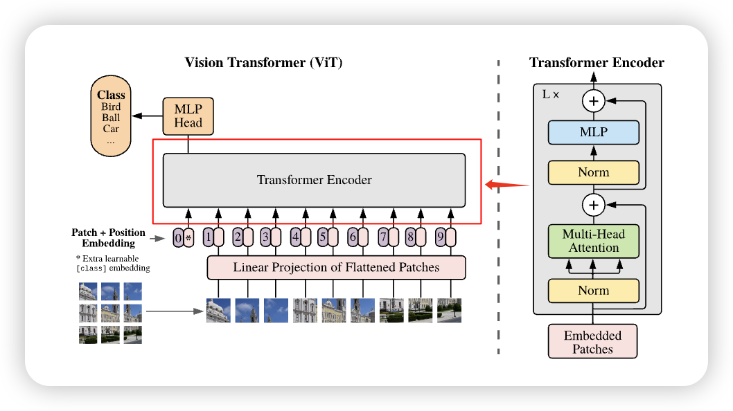
它的整体架构以及工作流程,如下图所示:

我们可以看到,ViT的整体流程可以分为以下几个步骤:
- Patchify: 将输入图像划分为若干大小相同的小块(Patch),并展开为一维序列。
- Linear Projection: 使用Linear Layer将每个 Patch 映射为固定维度的Hidden Embedding。
- 加入
[CLS]标记: 在序列开头添加一个特殊的[CLS]token,用于表示整张图像的全局语义。 - 位置编码: 为每个向量添加可学习的位置嵌入(Position Embedding),保留空间位置信息。
- Transformer Encoder: 将上述序列输入 Transformer Encoder,以捕捉全局依赖关系。
- 分类头(MLP Head): 最终通过一个MLP分类头输出图像所属的类别。
相对于 Transformer ,ViT 的主要区别在于:
- 增加了一个 Patchify 步骤,将图像划分为若干小块并转化为序列输入;
- 将原本的Sinusoidal position embedding替换为可学习的位置嵌入(Learned position embedding);
- 在最后额外添加了一个分类头(Classification head),用于完成图像分类任务。
我们之前已经学习过了什么是Transformer建议忘记了的同学再去回顾一下,我们就不多重复了。 我们首先来看如何进行Patch Embedding ,然后是Position Embedding,最后是Transformer Encoder Block。
2.1 Patch Embedding
在Transformer这一篇,我们了解到,它是作用于Sequence Modeling的, text就是很自然的Sequence Model,很显然,Image不是 Sequence的, 它有长(\(H\))和宽(\(W\))。很直观的第一种想法就是,将图片直接展开,从二维 \((3, H, W)\) 展开成一维的 \((3 \times H \times W)\). 这样我们就得到的图片的 Sequence Model。如下图 Figure 2 所示
这种方法有一种明显的问题就是:Sequence的长度太长。 举个例子,对于 \(3\times 256 \times 256\) 的图片,我们有 \(256 \times 256 = 65,336\) 个tokens,通过这种方法,所需要的训练时长很长 (在Transformer 这一节,我们了解过,Attention的时间复杂度是 \(\mathcal{O}(n^{2}d)\))。
另一个问题是:
所以我们很自然的想到:如果把相邻的pixels和在一组,组成一个patch,这样不就既减少了tokens的数量,又用到了pixel之间的correlation。这就是Vision Transformer的Patch Embedding。
The standard Transformer receives as input a 1D sequence of token embeddings. To handle 2D images, we reshape the image \(x \in \mathbb{R}^{H \times W \times C}\) into a sequence of flattened 2D patches\(x \in \mathbb{R}^{N \times (P^{2} \times C)}\), where (\(H, W\)) is the resolution of the original image, \(C\) is the number of channels, (\(P, P\)) is the resolution of each image patch, and \(N = HW/P^{2}\) is the resulting number of patches, which also serves as the effective input sequence length for the Transformer. The Transformer uses constant latent vector size \(D\) through all of its layers, so we flatten the patches and map to \(D\) dimensions with a trainable linear projection. We refer to the output of this projection as the patch embeddings. An Image is Worth 16x16 Words- Transformers for Image Recognition at Scale, p.3
有了Patch之后,我们就将图片从 \((H, W, C)\) 变成了 \((N, P, P, C)\), 其中 \(N = \frac{H \times W}{P^{2}}\)。 我们来看看代码怎么实现:
# Load Image and resize it to certain size
image_path = IMAGE_PATH
img_bgr = cv2.imread(image_path)
img_resized = cv2.resize(img_bgr, (IMAGE_SIZE, IMAGE_SIZE), interpolation=cv2.INTER_AREA)
img = cv2.cvtColor(img_resized, cv2.COLOR_BGR2RGB)

# Patchify
patches = einops.rearrange(
     img, "(h ph) (w pw) c -> (h w) ph pw c", ph=PATCH_SIZE, pw=PATCH_SIZE
)
通过这个Patchify之后,我们将图片分成了 \(\left( \frac{H}{P} \times \frac{W}{P}, P, P, C \right)\) 个Patches
接下来,我们将每个Patch 展开成一个向量,变成 \((N, P^{2} \times C)\),然后传入一个Linear Layer,将其映射到一个隐藏空间,变成 \((N, d_{model})\)。 这样,我们就得到了Transformer可以接受的输入。
flat_patch = einops.rearrange( patches, "n ph pw c -> n (ph pw c)")

mlp = nn.Linear(PATCH_SIZE * PATCH_SIZE * 3, d_model)
patch_embedding = mlp(flat_patch)
通过这种方法,我们就得到了Transformer可以接受的任意长度的输入。不过在实际操作中,我们并不会用以上的方式,而是用一个卷积层来实现这个Patch Embedding的过程。原因有二:
- 效率更高: 将Patchify + Flatten + Linear 合成一个卷积层,可以减少中间的内存读写,提高计算效率。
- 代码更简洁: 用一个卷积层就可以实现所有的功能,代码量更少,更易读懂。
如果我们用一个 卷积层,参数设置为:
kernel_size = PATCH_SIZE(卷积核覆盖一个 patch)stride = PATCH_SIZE(不重叠地移动,相当于切 patch)in_channels = 3(RGB 图片的通道数)out_channels = d_model
那么卷积会:
- 把输入图片分成
PATCH_SIZE x PATCH_SIZE的不重叠块(因为 stride = kernel_size)。 - 对每个 patch 做一次线性映射(因为卷积本质上就是对局部区域做加权求和,相当于 Linear)。
- 输出的 shape 自动就是 (batch, num_patches, d_model)。
这正好等价于 切 patch + flatten + Linear 的组合.
代码如下:
class PatchEmbedder(nn.Module):
    def __init__(self, config: ModelConfig):
        super().__init__()
        self.config = config
        self.num_patches_per_side = config.image_size // config.patch_size
        self.num_patches = self.num_patches_per_side**2

        self.proj = nn.Conv2d(
            in_channels=config.num_channels,
            out_channels=config.d_model,
            kernel_size=config.patch_size,
            stride=config.patch_size,
        )

    def forward(self, x: torch.Tensor):
        # x: (B, C, H, W)
        x = self.proj(x)  # (B, D, H/P, W/P)
        x = x.flatten(2)  # (B, D, N)
        x = x.transpose(1, 2)  # (B, N, D)
        return x
用卷积的好处,除了可以更高效的实现Patch Embedding,代码更加简洁之外,我们还可以通过改变 stride 来使一些Patch Overlapping,获得一个多尺度的结构。(尽管这个在ViT中没有提到,但是我觉得我们可以利用这一点)
NOTE: 关于Patch Embedding
可以补一句点明:“ViT 原版用 non-overlap patch,后续很多工作会用 overlap/conv stem 来补 inductive bias”。 我们之后会了解这一类变体。
我们计算一下,通过这种方法,可以减少多少Tokens的数量:
\[ \text{Number of Tokens} = \frac{H \times W}{P^{2}} \tag{1}\]
| Method | Number of Tokens | Attention Complexity |
|---|---|---|
| Flatten Image | \(224 \times 224 = 50,176\) | \(\mathcal{O}(n^{2}d) = \mathcal{O}(50,176^{2}d)\) |
| Patchify (\(P=8\)) | \(\frac{224 \times 224}{8^{2}} = 784\) | \(\mathcal{O}(n^{2}d) = \mathcal{O}(784^{2}d)\) |
| Patchify (\(P=16\)) | \(\frac{224 \times 224}{16^{2}} = 196\) | \(\mathcal{O}(n^{2}d) = \mathcal{O}(196^{2}d)\) |
| Patchify (\(P=32\)) | \(\frac{224 \times 224}{32^{2}} = 49\) | \(\mathcal{O}(n^{2}d) = \mathcal{O}(49^{2}d)\) |
从 Table 1 可以看出,通过Patchify,我们可以大大减少Tokens的数量,从而降低Attention的计算复杂度。这也是ViT能够在图像分类任务中取得成功的一个重要原因。不过,Patch Size的选择也是一个trade-off,过大可能会丢失细节信息,过小则会增加计算量。ViT原版使用的是 \(P=16\),即每个patch包含 \(16 \times 16\) 的像素。
TL;DR
ViT 的核心改动只有两步:patchify(切块)+ embedding(线性投影),其余几乎就是原封不动的 Transformer Encoder
2.2 Position Encoding
将图片转化为 Transformer 的输入之后,接下来Transformer中的另一个组件就是传入 Position Information。 我们知道在中,他们用的是 Sine-cosine position embedding,在那篇文章中,我们也提到了,还存在其他不同的Position Encoding的办法,ViT用的就是另一种办法,Learned Position Embedding。Learned Position Embedding的方法很简单,也很好理解,对于每一个位置,我们给他一个index,将这个index传入一个 Embedding Matrix, 我们就得到一个Position Embedding。不过与Token Embedding不同的是,我们会用到所有的Position,也整个matrix, 所以我们不用定index,直接定义整个Embedding,然后将它传入Transformer中。
class PosEmbedder(nn.Module):
    def __init__(self, config: ModelConfig):
        super().__init__()

        self.position_embeddings = nn.Parameter(
            torch.randn(1, (config.image_size // config.patch_size) ** 2 + 1, config.d_model)
        ) # +1 for cls token

        self.cls_token = nn.Parameter(torch.randn(1, 1, config.d_model))

    def forward(self, x: torch.Tensor):
        B = x.shape[0]
        cls_tokens = self.cls_token.expand(B, 1, -1)
        x = torch.cat((cls_tokens, x), dim=1)

        x = x + self.position_embeddings
        return x
Question: 为什么ViT要用Learned Position Embedding?
为什么ViT要用Learned Position Embedding呢?在ViT这篇文章中,他们尝试过不同的Position Embedding,比如:
- No Positional Information
- 1-dimensional Positional Embedding
- 2-dimensional Positional Embedding
- Relative Positional Embedding
发现,除了No Positional Information之外,其余3种在Image Classification中的表现,都是差不多的。
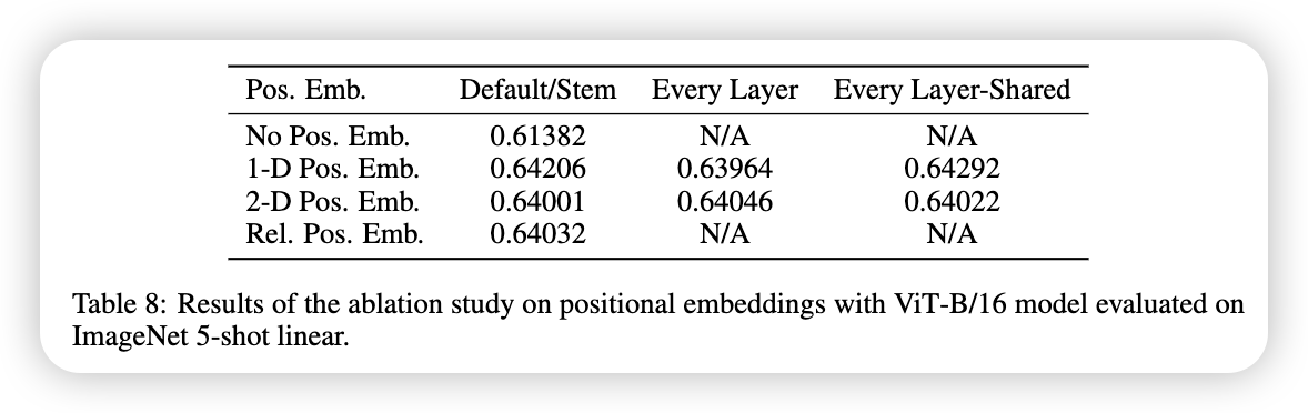
论文中表示,可能是因为所需要的Position的信息较小,对于不同种类的Position Embedding的方法,学习这个Position Information的能力,都是差不多的。
We speculate that since our Transformer encoder operates on patch-level inputs, as opposed to pixel-level, the differences in how to encode spatial information is less important. More precisely, in patch-level inputs, the spatial dimensions are much smaller than the original pixel-level inputs, e.g., \(14 \times 14\) as opposed to \(224 \times 224\), and learning to represent the spatial relations in this resolution is equally easy for these different positional encoding strategies. An Image is Worth 16x16 Words- Transformers for Image Recognition at Scale, p.18
不过,尽管Position的方法不重要,但是不同的训练参数,还是会影响到学习到的Position Information, 下图所示:
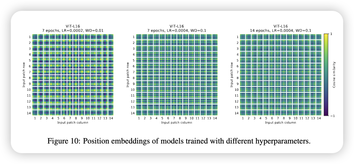
从图中看到,不同的训练参数,学习到的Position Information是不同的。
2.2.1 Position Interpolation
当我们有了一个Pre-Training的模型,我们想用它Fine-Tuning到一个不同图片大小的数据库,我们改怎么做呢?
第一个方法当然是,Resize 我们的图片,到ViT Pre-training的图片大小,但是,这个能导致较大的图片,失去很多细节。如果我们想保持图片的大小不变,同时让模型训练,我们就需要Extend Position Encoding,因为当Patch Size不变,图片大小变了的话,产生的Number of Patches 也是会改变的,我们需要做的是: 找到一种方法,增大或者减小Position的数量。 这就是所谓的Position Interpolation。
The Vision Transformer can handle arbitrary sequence lengths (up to memory constraints), however, the pre-trained position embeddings may no longer be meaningful. We therefore perform 2D interpolation of the pre-trained position embeddings, according to their location in the original image An Image is Worth 16x16 Words- Transformers for Image Recognition at Scale, p.4
我们可以把Position Embedding看成是\(\sqrt{Number of Patches} \times \sqrt{Number of Patches} \times dim\)的一张图像,那么当我们改变图片的大小,产生的patch数量也改变了,我们就可以通过对Position Embedding进行二维插值(2D Interpolation),来得到新的Position Embedding。
我们来看看代码是怎么实现Position Interpolation的:
def interpolate_pos_encoding(self, x, w, h):
    npatch = x.shape[1] - 1
    N = self.pos_embed.shape[1] - 1
    if npatch == N and w == h:
        return self.pos_embed
    class_pos_embed = self.pos_embed[:, 0]
    patch_pos_embed = self.pos_embed[:, 1:]
    dim = x.shape[-1]
    w0 = w // self.patch_embed.patch_size
    h0 = h // self.patch_embed.patch_size

    patch_pos_embed = F.interpolate(
        patch_pos_embed.reshape(
            1,
            int(math.sqrt(N)),
            int(math.sqrt(N)),
            dim
        ).permute(0, 3, 1, 2),
        scale_factor=(w0 / math.sqrt(N), h0 / math.sqrt(N)),
        mode='bicubic',
    )
    patch_pos_embed = patch_pos_embed.permute(0, 2, 3, 1).view(1, -1, dim)
    return torch.cat((class_pos_embed.unsqueeze(0), patch_pos_embed), dim=1)
需要注意的是代码的第6行和返回值,我们需要将位置编码分成两部分,一部分是 [CLS] token 的位置编码,另一部分是patch的位置信息。我们只对patch的位置信息进行插值,最后再将 [CLS] token 的位置编码和新的patch位置编码拼接起来。
TL;DR: 2D interpolation of the pre-trained position embeddings
ViT 在预训练时,通常用固定输入分辨率(比如 224×224) → 生成固定数量的 patch(比如 16×16 patch → 196 个 patch)。但在 fine-tuning 时,输入图片可能大小不一样,比如 384×384,这时 patch 数量就变了。这会导致原本的 位置编码 (position embeddings) 和新的 patch 数量对不上。解决办法:对预训练好的位置编码做 二维插值 (2D interpolation),根据 patch 在原图中的空间位置,把位置编码拉伸/缩放到新的分辨率。
2.3 [CLS] Tokens & MLP Head
在Transformer中,我们了解到:每输入一个token,Transformer会输出对应的token。这就是说,对于每个patch,Transformer会输出对应的Tokens,那么,我们应该选择哪一个token作为我们图片的表示呢。 BERT (Devlin et al. 2019), 用了一个 [CLS], 来表示一个句子。同理,我们也可以添加一个 [CLS] token, 来表示一张图片。同时,对于 [CLS] token, 我们也要在给他一个表示位置的信息。这就是为什么在Position Encoding上,我们有 (config.image_size // config.patch_size) ** 2 + 1, 位置信息,其中 +1 就是 [CLS] 的位置信息。
TL;DR: [CLS] Token
[CLS] token 的作用就是用来聚合所有的Patch的消息,然后用来Image 的Representation。
我们想一下,除了加一个 [CLS] token,之外,我们还有其他办法来表示图片吗。有一种很自然的方法就是,将所有的patch的消息收集起来,然后去一个平均值来表示这个图片。类似于传统的ConvNet我们可以通过 AvgPooling 来实现。 不过论文中提到, 对于两种不同的Image Representation,需要有不同的Learning Rate 来训练这个网络。 通过下图,我们看到,不用的收集信息的方法,需要不同的learning rate
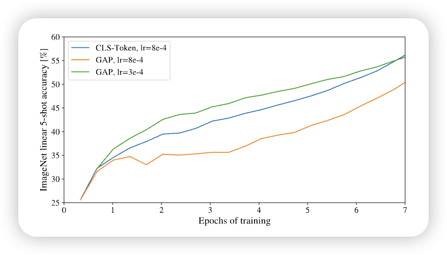
结构上二者都可行,但需要不同 LR / recipe。 实践里很多实现默认用 CLS(与 BERT 对齐、下游更统一),也有用 GAP 的变体比如我们接下来要学的 Swin Transformer (Liu et al. 2021)
An initial attempt at using only image-patch embeddings, globally average-pooling (GAP) them, followed by a linear classifier—just like ResNet’s final feature map—performed very poorly. However, we found that this is neither due to the extra token, nor to the GAP operation. Instead, the difference in performance is fully explained by the requirement for a different learning-rate, An Image is Worth 16x16 Words- Transformers for Image Recognition at Scale, p.17
有了Image Represent之后,我们只需要将这个Representation传入一个简单的MLP,我们就可以得到一个Classifier。MLP的输入是hidden dim,输出则是我们Number of Classes。不同的Index 表示不同的Classses。
Both during pre-training and fine-tuning, a classification head is attached to \(\mathrm{z}_{L}^{0}\). The classification head is implemented by a MLP with one hidden layer at pre-training time and by a single linear layer at fine-tuning time. An Image is Worth 16x16 Words- Transformers for Image Recognition at Scale, p.3
class MLPHead(nn.Module):
    def __init__(self, config: ModelConfig):
        super().__init__()
        self.fc1 = nn.Linear(config.d_model, config.d_model)
        self.fc2 = nn.Linear(config.d_model, config.num_classes)
        self.dropout = nn.Dropout(config.dropout_rate)

    def forward(self, x: torch.Tensor):
        cls = x[:, 0, :]
        cls = self.dropout(F.relu(self.fc1(cls)))
        cls = self.fc2(cls)

        return cls
2.4 Transformer Encoder Block
至此,我们已经讲完了ViT, 与Transformer的主要不同之处。接下来,就是Transformer的Encoder。
这部分,和Transformer原本的Encoder很类似,只不过有几处不同:
- Pre-Norm: 在ViT同,输入先进行一个LayerNorm,然后在传入MHA或者MLP中,反观在Transformer原本的Encoder中,我们是先将MHA或者MLP的输出与输入加在一起,之后再进行一个Normalization。这叫做Post-Norm,
\[ \begin{split} \text{Post-Norm:} \quad x_{l} &= \mathrm{Norm}(x_{l-1} + \mathrm{MHA}(x_{l-1})) \\ \text{Pre-Norm:} \quad x_{l} &= x_{l-1} + \mathrm{MHA}(\mathrm{Norm}(x_{l-1})) \end{split} \tag{2}\]
Pre-Norm的好处是,Gradient可以不受干扰的直接流过残差连接(residual connection),而Post-Norm则会有一些干扰,导致训练不稳定。ViT使用Pre-Norm来提高训练的稳定性。
- MLP的实现:在Transformer Encoder中,用的是
ReLU, 而在ViT中,用的是GELU
除此之外,其他部分都是一样的。一下是ViT Encoder的实现:
class EncoderBlock(nn.Module):
    def __init__(self, config: ModelConfig):
        super().__init__()
        self.mha = MHA(config)
        self.ffn = FFN(config)
        self.norm1 = LayerNorm(config.d_model)
        self.norm2 = LayerNorm(config.d_model)

    def forward(self, x: torch.Tensor):
        attn, _ = self.mha(self.norm1(x))
        x = x + attn
        x = x + self.ffn(self.norm2(x))

        return x
2.4.1 Multi-Heads Attention
还有一个就是Attention模块,Attention模块与Transformer的是一模一样,在这里就不过多的赘述了。
class MHA(nn.Module):
    def __init__(self, config: ModelConfig):
        super().__init__()
        self.num_heads = config.num_heads
        self.d_model = config.d_model
        assert config.d_model % config.num_heads == 0, "d_model must be divisible by num_heads"
        self.d_k = config.d_model // config.num_heads

        self.qkv_linear = nn.Linear(config.d_model, config.d_model * 3)
        self.out_linear = nn.Linear(config.d_model, config.d_model)

        self.attention_dropout = nn.Dropout(config.attention_dropout_rate)

    def forward(self, x: torch.Tensor):
        B, N, C = x.shape  # Batch size, Number of tokens, Embedding dimension

        q, k, v = (
            self.qkv_linear(x).reshape(B, N, 3, self.num_heads, self.d_k).permute(2, 0, 3, 1, 4).unbind(0)
        )

        scores = torch.matmul(q, k.transpose(-2, -1)) / torch.sqrt(
            torch.tensor(self.d_k, dtype=torch.float32)
        )  # (B, num_heads, N, N)
        attn_weight = torch.softmax(scores, dim=-1)  # (B, num_heads, N, N)
        attn = self.attention_dropout(attn_weight)

        context = torch.matmul(attn, v)  # (B, num_heads, N, d_k)
        context = context.transpose(1, 2).reshape(B, N, C)  # (B, N, d_model)

        out = self.out_linear(context)  # (B, N, d_model)

        return out, attn_weight
2.5 CNN vs. ViT: Inductive bias
至此,我们已经介绍完了Vision Transformer,我们来从Inductive Bias的方面,看看 CNN 和 ViT 有什么不同
NOTE: Inductive Bias
在深度学习里,Inductive Bias(归纳偏置)是指模型在学习之前,因结构或设计而自带的假设或先验 ,比如 Convolution Layer, 它就是假设相邻的pixel之间,是有一定联系的,因此可以用一个Kernel来将学习这些关系。
对于图像来说,常见的先验就是:
- 局部像素是相关的(locality)
- 相邻区域的模式有规律(2D neighborhood)
- 物体无论出现在图像哪里,识别方式应该一样(Translation Equivariance)
那么,CNN 的结构怎么体现这些偏置?
- 局部性 (Locality):
- 卷积核(例如 \(3 \times 3\))只和局部像素打交道,而不是全图。
- 这意味着模型“相信”图像的重要特征来自局部邻域,而不是遥远区域。
- 二维邻域结构 (2D structure):
- 卷积操作是沿着 图像的二维网格进行的,天然利用了图像的行列结构。
- 这和文本(序列 1D)不一样,CNN 明确知道输入是 2D 排列的。
- 平移等变性 (Translation equivariance):
- 卷积核的参数在整张图共享。
- 所以猫在左上角还是右下角,卷积核都能检测到“猫耳朵”。
- 这让 CNN 自动具有“识别位置无关”的能力。
这些性质不是模型通过训练学出来的,而是因为卷积操作本身的数学结构就带来的(也是我们人为设计的):
- kernel 的局部连接 → 局部性
- kernel 滑动覆盖全图 → 平移等变性
- 操作在二维空间定义 → 邻域结构
所以,哪怕我们不给 CNN 喂太多数据,它也会利用这些偏置去学习特征。
而对于 ViT 来说,其归纳偏置非常弱,几乎完全依赖数据和训练来学习,不过它也有利用了一些图片的Inductive Bias:
- Patch 切分 (Patchification)
- ViT 唯一的“图像先验”之一就是把输入图片切成 patch
- 这一操作隐含了:图像是一个二维结构,可以被分块处理。
- 位置编码 (Positional Embeddings)
- Transformer 本身只处理序列,没有空间结构的概念。
- ViT 通过加位置编码告诉模型 patch 在图像中的相对位置。
- 在输入分辨率变化时,会做 二维插值 (2D interpolation) 来适配,这也是一种人工引入的 2D 先验。
- 其他部分
- 除了以上两点,ViT 的注意力机制是 全局的 (global),没有局部性约束。
- 没有像 CNN 那样内置的平移等变性或局部邻域结构。
这样就是为什么ViT需要更多数据和计算才能学到同样的空间归纳规律。
ViT is Data-Hungry because it has very weak inductive bias, relying on the data to learn spatial relationships, while CNNs have strong built-in biases that help them learn from less data.
2.6 ViT Model Variants
ViT 有3种不同的基本变形, 如下表:
| Variant | #Layers | Hidden Dim (d_model) | MLP Dim (d_ff) | #Heads | #Params |
|---|---|---|---|---|---|
| ViT-Base (ViT-B/16) | 12 | 768 | 3072 | 12 | 86M |
| ViT-Large (ViT-L/16) | 24 | 1024 | 4096 | 16 | 307M |
| ViT-Huge (ViT-H/14) | 32 | 1280 | 5120 | 16 | 632M |
ViT的名字通常表示为: ViT-L/16: 意思是,ViT-Large,然后用的16 Patch Size。 需要注意的是,Patch Size越大,我们得到的tokens就越少,也就是需要更少的训练时实现, 但通常需要更大的图片来训练。
2.7 Experiment
我们先来看看原论文是如何训练的:
- 预训练(所有模型,包括 ResNet):作者统一使用 Adam(\(\beta_{1} = 0.9, \beta_{2}=0.999\)),batch size = 4096,并使用较大的 weight decay = 0.1。作者指出这对所有模型的迁移表现都有帮助
- 学习率策略:采用线性 warmup + 线性 decay(细节见 Appendix B.1)。
- 微调(fine-tuning):对所有模型统一改用带 momentum 的 SGD,batch size 512.
- 权重平均:同时使用 Polyak averaging(指数滑动平均,系数 0.9999)以进一步提升效果。
接下来,我们来训练我们定义的ViT。具体的代码可以在 这里 查看。
2.7.1 Dataset
我们用CIFAT-10的训练集来训练ViT。
WARNING: Limited of Dataset
我们之前提到了ViT要在大规模的数据集上才可以发挥它的能力,由于资源有限,我们只在这展示ViT的训练流程,在了解了这个训练流程之后,很容易拓展到其他的大数据集。
IMG_MEAN = [0.4914, 0.4822, 0.4465]
IMG_STD = [0.2470, 0.2435, 0.2616]
IMG_SIZE = 32


data_transform = transforms.Compose(
    [
        transforms.Resize(
            (IMG_SIZE, IMG_SIZE),
            interpolation=transforms.InterpolationMode.BILINEAR,
        ),
        transforms.RandomHorizontalFlip(),
        transforms.ToTensor(),
        transforms.Normalize(IMG_MEAN, IMG_STD),
    ]
)

train_dataset = torchvision.datasets.CIFAR10(
    root=train_config.data_dir, download=True, train=True, transform=data_transform
)
if train_config.debug:
    train_dataset = torch.utils.data.Subset(train_dataset, range(1000))


dataloader = DataLoader(
    train_dataset,
    batch_size=train_config.batch_size,
    shuffle=True,
    num_workers=4,
    pin_memory=True if train_config.device.type == "cuda" else False,
)
2.7.2 Optimizer & Loss Function
论文中应用了 Adam Optimizer,我们在此也用Adam。因为我们训练的是Image Classification Task,所以损失函数是是Cross Entropy Loss:
2.7.3 Result
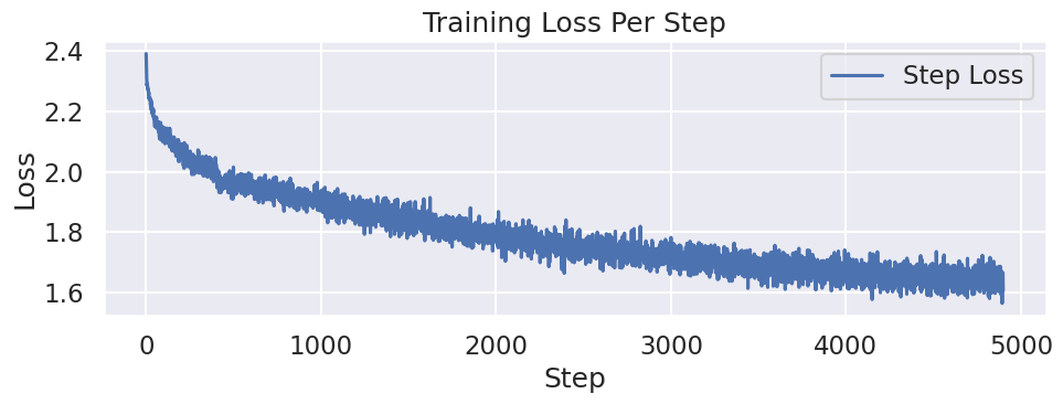
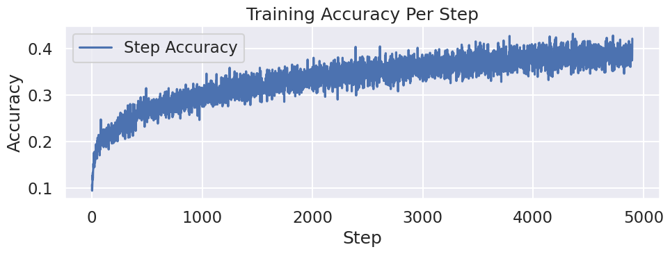
我们来看看,这个Toy ViT 究竟训练的怎么样:
N_ROWS = 4
N_COLS = 8
N_IMGS = N_ROWS * N_COLS
test_dataset = torchvision.datasets.CIFAR10(
    root=train_config.data_dir,
    download=True,
    train=False,
)
IDX_TO_CLASS = {v: k for k, v in test_dataset.class_to_idx.items()}

org_imgs, true_labels = test_dataset.data[:N_IMGS], test_dataset.targets[:N_IMGS]
transformed_imgs = torch.stack([data_transform(Image.fromarray(img)) for img in org_imgs])
pred_labels = model(tensor_to_device(transformed_imgs, device=train_config.device)).argmax(dim=1).cpu()


fig, axes = plt.subplots(N_ROWS, N_COLS, figsize=(N_COLS * 2, N_ROWS * 2))
for i in range(N_ROWS):
    for j in range(N_COLS):
        idx = i * N_COLS + j
        axes[i, j].imshow(org_imgs[idx])
        axes[i, j].axis("off")
        if true_labels[idx] == pred_labels[idx].item():
            axes[i, j].set_title(
                f"{IDX_TO_CLASS[true_labels[idx]]} (Pred: {IDX_TO_CLASS[pred_labels[idx].item()]})",
                fontsize=10,
                color="green",
            )
        else:
            axes[i, j].set_title(
                f"{IDX_TO_CLASS[true_labels[idx]]} (Pred: {IDX_TO_CLASS[pred_labels[idx].item()]})",
                fontsize=10,
                color="red",
            )
plt.tight_layout()
plt.show()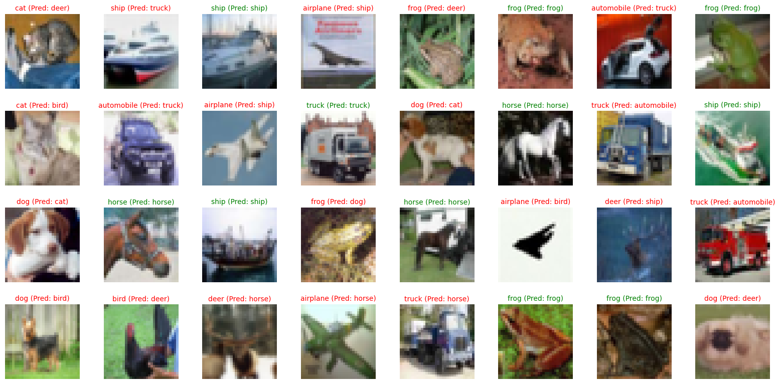
我们也可以看看Attention Map的
N_ROWS = 4
N_COLS = 8
N_IMGS = N_ROWS * N_COLS
test_dataset = torchvision.datasets.CIFAR10(
    root=train_config.data_dir,
    download=True,
    train=False,
)
IDX_TO_CLASS = {v: k for k, v in test_dataset.class_to_idx.items()}

org_imgs, true_labels = test_dataset.data[:N_IMGS], test_dataset.targets[:N_IMGS]
transformed_imgs = torch.stack([data_transform(Image.fromarray(img)) for img in org_imgs]).to(
    train_config.device
)

# pred_labels = model(tensor_to_device(transformed_imgs, device=train_config.device)).argmax(dim=1).cpu()
TARGET_LAYER = 5  # 0-based index
HEAD = 2
GAMMA = 0.7
FLOOR = 0.15


def to_vit_attention_vis(img_uint8, attn_map, gamma=0.7, floor=0.15):
    """
    gamma:     >0, smaller -> sharper spotlight
    floor:     how visible the dark region is (0 = pure black background)
    """
    img = img_uint8.astype(np.float32) / 255.0

    # normalize attention to [0,1]
    a = attn_map.astype(np.float32)
    a = a - a.min()
    a = a / (a.max() + 1e-6)

    # make it more "spotlight-like"
    a = a**gamma  # sharpen
    a = floor + (1 - floor) * a  # keep some visibility outside
    a = np.clip(a, 0, 1)

    return img * a[..., None]  # darken outside attention


model.eval()
x = model.backbone.patch_embedder(transformed_imgs)
x = model.backbone.pos_embedder(x)
for i in range(TARGET_LAYER):
    x = model.backbone.encoder_layers[i](x)

_, attn_weights = model.backbone.encoder_layers[TARGET_LAYER].mha(
    model.backbone.encoder_layers[TARGET_LAYER].norm1(x)
)
if HEAD >= 0:
    attn_weights = attn_weights[:, HEAD, 0, 1:]  # (B, N)
else:
    attn_weights = attn_weights.mean(dim=1)[:, 0, 1:]  # (B, N)

# Reshape attention weights to (B, H, W)
num_patches_per_side = model_config.image_size // model_config.patch_size
attn_maps = attn_weights.reshape(-1, num_patches_per_side, num_patches_per_side)  # (B, H, W)

# Upsample attention maps to image size
attn_maps_upsampled = F.interpolate(
    attn_maps.unsqueeze(1),
    size=(model_config.image_size, model_config.image_size),
    mode="bilinear",
    align_corners=False,
).squeeze(1)  # (B, H, W)

# Move attention map to CPU for visualization
attn_maps_upsampled = attn_maps_upsampled.cpu().detach().numpy()

# Visualize Overlaid Attention Maps
fig, axes = plt.subplots(N_ROWS, N_COLS, figsize=(N_COLS * 2, N_ROWS * 2))
for i in range(N_ROWS):
    for j in range(N_COLS):
        idx = i * N_COLS + j
        vis = to_vit_attention_vis(
            org_imgs[idx],
            attn_maps_upsampled[idx],
            gamma=GAMMA,
            floor=FLOOR,
        )

        axes[i, j].imshow(vis)
        axes[i, j].axis("off")
        if true_labels[idx] == pred_labels[idx].item():
            axes[i, j].set_title(
                f"{IDX_TO_CLASS[true_labels[idx]]} (Pred: {IDX_TO_CLASS[pred_labels[idx].item()]})",
                fontsize=10,
                color="green",
            )
        else:
            axes[i, j].set_title(
                f"{IDX_TO_CLASS[true_labels[idx]]} (Pred: {IDX_TO_CLASS[pred_labels[idx].item()]})",
                fontsize=10,
                color="red",
            )
plt.tight_layout()
plt.suptitle(
    f"Attention Maps Over Images On Layer {TARGET_LAYER}  {'Head ' + str(HEAD) if HEAD >= 0 else 'Avg Head'}",
    y=1.02,
)
plt.show()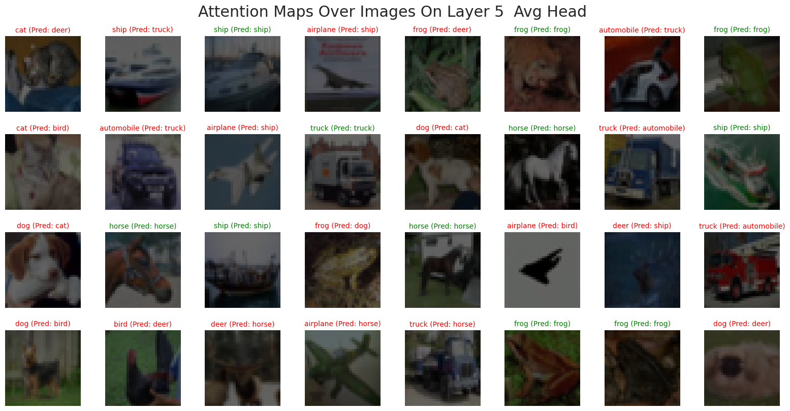
2.7.4 Training Recipe
接下来我提供几个可能的提升Accuracy的方法(由于时间现实,暂时没有能实现,有兴趣的读者欢迎自行尝试):
- 优化器:AdamW(而非 Adam)+ weight decay
- 学习率策略:warmup + cosine,batch size 对 LR 的线性缩放规则
- 增强:RandAugment / Mixup / CutMix
- 正则:DropPath(stochastic depth)、Label smoothing
TIP: ViT 训练常见组合
AdamW + cosine + warmup + strong aug(RA/Mixup/CutMix)+ DropPath + label smoothing
2.7.5 Training Summary
从实验结果来看,这个 toy ViT 的表现确实不算理想,甚至不如一个简单的卷积网络。这其实在预期之内:ViT 的归纳偏置更弱(缺少卷积的局部性与平移等变性),在数据量较小、训练 recipe 不够强的情况下更容易欠拟合或泛化不足,因此很难在 CIFAR-10 这类小规模数据上占到便宜。
比较“反直觉”的是,我们可视化得到的 Attention Map 几乎接近均匀分布,而不是像原论文那样呈现出更清晰的语义聚焦(例如对物体区域的注意力更强):
![]()
一种合理的解释是:我们的输入分辨率只有 (\(32\times32\)),在常见 patch 设置下 token 数量非常有限(例如 (\(P=4\)) 时也只有 (\(8\times8=64\)) 个 patch)。在这种低分辨率、低 token 数的设定里,每个 token 覆盖的区域相对“粗”,并且早期训练阶段模型往往更倾向于学习全局平均的相关性来最小化损失,导致注意力权重看起来更平均。另一个注意的点就是:单层注意力权重本身未必等价于“可解释性”,即使模型在做出正确决策,也可能出现注意力图不够尖锐的现象。
如果希望得到更有信息量的可解释结果,通常有两条更稳妥的路径:
- 使用更可靠的可解释方法,例如 Grad-CAM (Selvaraju et al. 2020),或者结合多层注意力的 Attention Rollout (Abnar and Zuidema 2020),而不是只观察某一层/某一头的 attention。
- 提高输入分辨率与训练规模(例如在 ImageNet 或更大数据上训练/预训练后再迁移),让模型有机会学习到更细粒度的空间结构与更稳定的语义对齐。
这里就不展开实现细节了,有兴趣的同学可以根据上述论文进一步尝试与对比。
3 Others
3.1 Self-Supervised Pre-Training
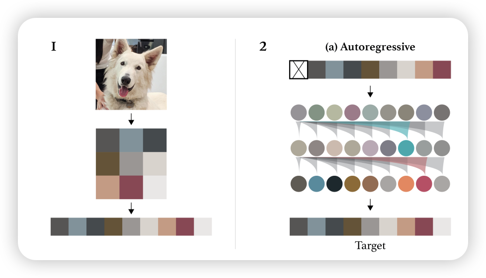
除了做 Image Classification,ViT 团队也尝试了自监督预训练(Self-Supervised Pre-Training)。他们采用了一种非常“类似于BERT(Devlin et al. 2019)”的思路:Masked Patch Prediction——先把图像切成 patch tokens,然后随机“腐蚀(corrupt)”一部分 token,让模型去预测被腐蚀部分的内容。
核心是把 ViT 当成“视觉版 BERT”:随机遮住(或替换)一部分 patch token,再预测被遮住 patch 的目标(这里用离散颜色作为预测标签)。
![]()
他们对 50% 的 patch embedding 做 corruption,并采用与 BERT 类似的 80/10/10 策略: - 80%:用一个可学习的 [mask] embedding 替换 - 10%:替换成另一块随机 patch 的 embedding - 10%:保持不变(但仍然作为预测目标)
这种设计的直觉是:既要让模型学会“根据上下文补全缺失信息”,又要避免模型过度依赖某一种固定的 mask 模式。
他们最终选择了一个非常轻量但有效的预测目标:
对每个被腐蚀 patch,预测其 3-bit mean color(一共 \(2^9 = 512\) 种颜色,也就是一个 512-way 分类问题)。
同时他们也对比过几种目标设定: 1) 只预测一个 mean 3-bit color(512 分类,1 个预测)
2) 把 16×16 patch 下采样成 4×4,再对每个小格预测 3-bit color(512 分类,16 个并行预测)
3) 直接对完整 patch 做像素级 L2 回归(RGB 通道上的密集回归)
结果比较有意思:三种方式都能带来不错效果,但 像素 L2 回归略差.
We employ the masked patch prediction objective for preliminary self-supervision experiments. To do so we corrupt 50% of patch embeddings by either replacing their embeddings with a learnable
[mask]embedding (80%), a random other patch embedding (10%) or just keeping them as is (10%). This setup is very similar to the one used for language by BERT. Finally, we predict the 3-bit, mean color (i.e., 512 colors in total) of every corrupted patch using their respective patch representations An Image is Worth 16x16 Words- Transformers for Image Recognition at Scale, p.14
后续的工作也说明了这种方法的可行性,比如SiMIM (Xie et al. 2022)
4 Key Concepts
| Content | Explain |
|---|---|
| Patchify | 把 \((H\times W)\) 图像切成 \((P\times P)\) 小块并展平,得到 token 序列,是 ViT 的核心“视觉→序列”接口。 |
| Patch Embedding | 用线性投影 (\(E\)) 把每个 patch 从 \((P^2C)\) 映射到 Transformer 维度 (\(D\))。 |
| [CLS] Token | 在序列前加入可学习 token,用其输出表示整图并接分类头。 |
| Positional Embedding | ViT 用可学习 1D 位置编码;分辨率变化时对位置编码做 2D 插值以适配新 token 网格。 |
| Pre-LN Transformer Encoder | LayerNorm 放在子层前,配合残差:MSA 和 MLP 交替堆叠。 |
| Inductive Bias | CNN 的局部性/平移等变性;ViT 归纳偏置更弱,更依赖数据规模与训练配方。 |
| Model Scaling (B/L/H) | Base/Large/Huge 三档参数与深度,patch 越小序列越长、计算更贵。 |
5 Q&A
5.1 Question 1
Question 1: 为什么 Vision Transformer 需要大规模预训练数据?
因为 ViT 缺乏卷积神经网络中的归纳偏置(inductive bias),例如局部性(locality)和平移不变性(translation equivariance),这些能力需要通过大量数据来学习。
5.2 Question 2
Question 2:Eq.(1) 里为什么要加 [CLS] token,它和全局平均池化有什么区别?
[CLS] token 给模型一个“专门聚合信息的槽位”,通过注意力主动从所有 patch 拉取信息;而 GAP 是被动平均。论文在附录对比过两者表现接近,但学习率等配方可能需要不同调整。arXiv+1
5.3 Question 3
Question 3:ViT 用 1D position embedding 不会丢掉 2D 结构吗?
丢掉了“显式 2D 归纳偏置”,但作者发现更复杂的 2D-aware 位置编码并没有带来显著收益;ViT 依靠数据与训练从头学习空间关系。真正需要 2D 的地方主要在分辨率迁移时的位置编码插值。arXiv+1
5.4 Question 4
Question 4:为什么论文强调“规模训练胜过归纳偏置”?
论文实验显示:小数据预训练时强 CNN(如 BiT ResNet)更稳;随着预训练数据从 ImageNet → ImageNet-21k → JFT-300M 增大,ViT 大模型的迁移性能显著提升并反超 CNN,说明对 ViT 而言数据规模是关键瓶颈。UofT Computer Science+1
5.5 Question 5
Question 5:patch size 选 16 还是 32 的主要权衡是什么?
patch 越小(如 16)→ token 数 NNN 越大 → 注意力更贵但细粒度更强;patch 越大(如 32)→ 更省算力但可能损失细节。论文也明确指出序列长度与 P2P^2P2 成反比,因此小 patch 更昂贵。
5.6 Question 6
Question 6:为什么 ViT 在小数据集上通常不如 CNN?
因为 CNN 通过卷积和权重共享内置了强先验,而 ViT 需要从数据中学习这些先验,在小数据条件下不够高效。
5.7 Question 7
Question 7:分辨率微调时为什么要对位置编码做 2D 插值?
因为 token 网格大小变了(NNN 变了),预训练的 EposE_{pos}Epos 不能直接对齐新位置;2D 插值让位置编码在空间上“平滑伸缩”,从而复用预训练知识。
5.8 Question 8
Question 8:为什么 ViT 需要把图像切成 patch,而不是直接把每个像素当 token?
像素级 token 会让序列长度变成 \(H \times W\),自注意力复杂度 \(\mathcal{O}(n^{2})\) 直接爆炸;patchify 把 NNN 降到 \(\frac{HW}{P^2}\),让标准全局注意力在可接受的算力下运行,同时保留端到端学习空间结构的能力。
6 Related resource & Further Reading
在了解了什么是Vision Transformer之后,我们可以看看这些还有那些提升,比如这篇文章,介绍了一些训练ViT的技巧
How to train your ViT? Data, Augmentation, and Regularization in Vision Transformers 论文中总节了三类改进策略:
| 类别 | 代表方法 | 效果 |
|---|---|---|
| 数据增强 (Data Augmentation) | RandAugment, Mixup, CutMix, Random Erasing | 提高泛化,抵消数据量不足 |
| 正则化 (Regularization) | DropPath(Stochastic Depth), Label Smoothing, Gradient Clipping | 稳定训练、防止过拟合 |
| 优化器与学习率调度 | AdamW + Cosine LR + Warmup | 对 ViT 特别关键 |
6.1 减少Tokens的技巧
6.1.1 Patch Merge
类似于 Swin Transformer(Liu et al. 2021) 的做法:在不同层将相邻 patch 合并(例如 2×2 → 1),减少 token 数,使模型层级化。
6.1.2 Pixel Shuffle
![]()
6.2 Vision Language Model
我们以及学习了ViT for computer Vision, Transformer for NLP, 接下来有什么办法让这两种模型结合起来呢? CLIP (Radford et al. 2021): 将 ViT 融合到 vision-language 预训练中。我们之后会学习这篇文章。
6.3 Video Transformer
在学习了如何将Transformer应用到Image中,我们可以更近一步,看看如何将Transformer应用到Video 模态中。ViViT(Arnab et al. 2021) 的提出,就是将Transformer应用到Video。中,我们之后会学习到这一篇。
6.4 Native Resolution
在ViT 中,我们需要将图片Resize到相同大小的图片,那我们就想不Resize,能不能直接训“不同大小/不同长宽比”的图? NaViT (Dehghani et al. 2023)提出每张图在“原始分辨率/原始长宽比”下切成 patch token 序列,然后把多张图的 token 序列“打包(packing)”到同一条固定长度序列里训练,用 attention mask 保证不同图片之间互不“串门”。
![]()
- Patch n’ Pack:把多张不同分辨率图片的 patch token 序列拼成一个定长 packed sequence,以减少 padding/resize 浪费
- Attention Mask:使用 block-diagonal mask,让同一张图的 token 才能互相 attention,不同图之间完全隔离
- 位置编码:采用 factorized(x/y 分解)位置编码,并可用 fractional 坐标提升对未见分辨率的泛化
7 Summary
恭喜你看到了这里,ViT的论文架构思想很简单,但就是这种大道至简的方式,才让它这个工作变得出彩。尽管如此,细看ViT的论文,还是有很多可学习的地方。接下来,我们来回顾一下。
在本章中,从已熟悉 Transformer 的前提出发,围绕 “如何将 Transformer 应用于计算机视觉” 这一核心问题,系统梳理了 Vision Transformer(ViT)的整体设计与实现思路。文章首先介绍了 ViT 的基本架构,说明其本质是将二维图像通过 Patchify 转化为一维序列,并结合 Patch Embedding、Position Embedding 与 [CLS] token,使图像能够被标准的 Transformer Encoder 处理。随后介绍了 Patch Embedding 的动机与实现:从像素级直接展开所带来的序列过长与计算复杂度问题出发,引出将相邻像素组合成 patch 的必要性,并给出了基于 einops 的直观实现以及使用 Conv2d 等价实现 的工程化写法。
在位置编码部分,对比了 ViT 中采用的 Learned Position Embedding 与传统 Transformer 的正余弦位置编码,并结合论文实验说明,在 patch-level 输入下,不同位置编码策略在图像分类任务中的性能差异并不显著;同时介绍了在 fine-tuning 到不同输入分辨率时,如何通过 二维插值(2D interpolation) 扩展预训练位置编码以适配新的 patch 数量。随后从表示学习的角度讨论了 [CLS] token 在 ViT 中的作用,并与全局平均池化(GAP)进行对比,指出两种方式的性能差异主要来源于训练时学习率等超参数设置,而非结构本身。
在模型结构层面,强调了 ViT Encoder 与原始 Transformer Encoder 的关键差异,包括 Pre-Norm 设计 以及使用 GELU 激活函数。接着从 Inductive Bias 的视角对比了 CNN 与 ViT:CNN 通过卷积天然引入局部性、二维结构和平移等变性等先验,而 ViT 的归纳偏置较弱,更多依赖数据和训练过程来学习这些空间规律,这也解释了 ViT 在小数据集上表现受限、但在大规模预训练条件下潜力显著的原因。最后,通过在 CIFAR-10 上训练一个 toy ViT 的实验,展示了模型的分类效果与注意力可视化,并分析了 attention map 接近均匀的现象可能与 低分辨率和数据规模有限 有关,同时给出了进一步改进与扩展的方向,为后续更高效注意力机制以及多模态、视频模型的学习奠定基础。
8 In the end
创作不易,如果你觉得内容对你有帮助,欢迎请我 喝杯咖啡/支付宝红包,支持我继续创作!你们的支持是我最大的动力! :)

9 Appendix
9.1 Axial Attention(轴向注意力)
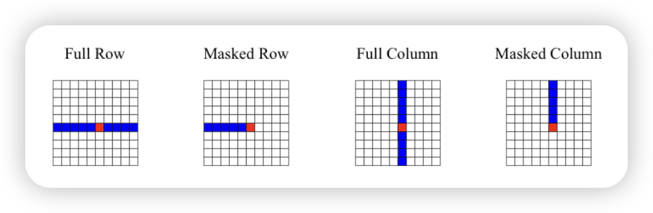
在处理 图像或视频 这类高维输入时,如果直接对所有像素做 全局 self-attention,复杂度是 \(\mathcal{O}(H^2 W^2)\)当图像很大时,这个代价太高。 核心想法:把二维 attention 拆成两次一维 attention(沿着图像的两个“轴”分别做)。 1. Row-wise Attention(行注意力) • 沿着水平方向(宽度轴 W)做注意力,每一行的像素互相关注。 • 复杂度:\(\mathcal{O}(H \cdot W^2)\)。 2. Column-wise Attention(列注意力) • 沿着垂直方向(高度轴 H)做注意力,每一列的像素互相关注。 • 复杂度: \(\mathcal{O}(W \cdot H^2)\)。
组合起来,相当于在 H 和 W 两个轴上都做了全局依赖建模。