Lecture 16 & 17: LLM Alignment SFT & RLVR（GRPO）

这节介绍了PPO， 以及DPO所存在的问题，并且引出了Reinforcement Learning from Verified Rewards (RLVR)的新方法GRPO。内容包括Advantage Function、Length Normalization关键技术细节，并通过DeepSeek-R1、Kimi 1.5和Qwen3等案例展示了GRPO在实际中的应用。而Lecture17则通过一个排序任务的具体例子，详细讲解了GRPO算法的实现细节，包括数据生成、奖励函数设计、模型架构以及训练过程，在这里就把两节课合成一节课来写。

在之前的课程中，我们学习了PPO以及DPO的算法，我们因此也从GPT得到了ChatGPT。但这距离现在的 Reasoning Model，还有一段距离。在这节课中，我们将学习新的一系列算法，也就是RLVR(Reinforcement Learning from Verified Rewards)，通过这些算法，我们可以从ChatGPT突破到ChatGPT-o1。

在了解RLVR之前，我们先来看一下，为什么不直接用PPO和DPO来做LLM的推理强化学习。

推荐阅读

对于想更深入了解 RL in LLM 的同学们，我推荐阅读我这一篇文章 Reinforcement Learning in LLM。在这篇文章中，我们系统地介绍了 LLM 中的强化学习，包括 PPO、DPO 以及 RLVR 的原理和实现细节。并且对比了不同的RLVR的算法，比如GRPO，GSPO，DAPO等。

1 Why NOT PPO & DPO ?

1.1 Why Not PPO?

PPO理论上就一个clip目标，但落地要处理很多组件, 包括：

• rollout采样/缓存、old logprob、ratio、clip、KL penalty/target KL
• advantage估计（GAE）、return计算

对LLM来说，rollout很贵（推理生成token），所以还会引入“采一次rollout，更新多次”的机制，这又把实现复杂度继续抬高。并且，最主要的问题是：

PPO通常需要一个 value function 来计算Advantage.

这意味着：

• 额外的模型（value model）+内存开销
• 额外的训练目标（value loss）

“Value model (memory hungry, involves additional tuning)”

1.2 Why Not DPO?

DPO的强项是偏好对比数据 \((p, y_i, y_j)\)，但在可验证奖励的推理RL里，数据常见是：

• 一个prompt，
• 一个回答，
• reward=0/1（对/错）或分数

数据不是天然的pairwise偏好，而是pointwise reward。另外，DPO常见使用方式偏Off-Policy：先收集对比数据，再训练。而推理RL通常更像在线：模型不断变强 → 不断rollout → 不断用最新策略生成新数据训练（on-policy味道更强）。GRPO/PPO天然适配这种循环。

2 What is RLVR?

RLVR (Reinforcement Learning from Verified Rewards) 是一类专门为 LLM 推理强化学习设计的算法。它们利用可验证奖励（例如数学题的对错）来优化模型的推理能力。 它的流程大致如下 Figure 1 (a)：

(a) Overview of RLVR

(b) Overview of RLHF

Figure 1: RLVR vs RLHF， RLHF 依赖人工偏好数据，而 RLVR 则利用可验证奖励进行训练。 RLVR 利用 Verified Rewards 直接优化模型的推理能力，而不需要额外的奖励模型。

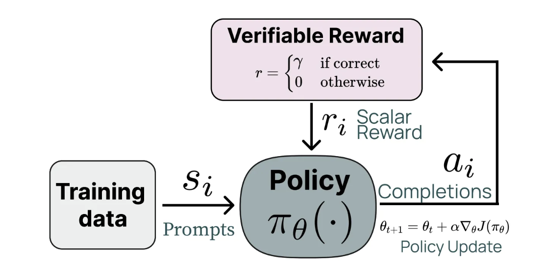
相比于RLHF，RLVR有以下优势：

• 直接利用可验证奖励：RLVR直接使用可验证的奖励信号（如数学题的对错），而不需要训练复杂的奖励模型。这简化了训练流程，减少了对高质量偏好数据的依赖。
• 对模型输出的严格约束：RLVR方法通常设计了专门的目标函数，确保模型在生成推理链时遵循逻辑和事实，从而提高了模型的可靠性和准确性。
• 更高的样本效率：通过利用可验证奖励，RLVR方法能够更有效地利用训练数据，提高模型的学习效率，减少所需的训练样本数量。

3 GRPO

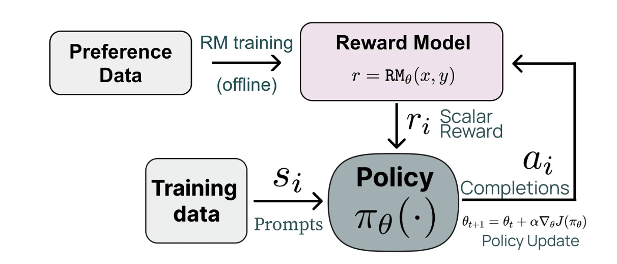
回顾了PPO和DPO在LLM推理RL上的局限后，我们来看GRPO(Shao et al. 2024)。GRPO与PPO的主要流程与区别如下：

Figure 2: 对比了 PPO 与 GRPO 的训练流程差异：
上半部分（PPO）中，策略模型在生成单个输出 \(o\) 后，分别通过Reward Model与Reference Model得到Reward \(r\) 与 KL 约束，并依赖Value Model预测的状态价值 \(v\)，再用 GAE 计算优势 A 来更新策略；
下半部分（GRPO）中，策略模型对同一提示 \(q\) 一次性采样一组输出 \(\{o_1,\dots,o_G\}\)，仅依赖冻结的Reward Model与Reference Model得到组内奖励 \(\{r_1, r_2, \dots, r_G\}\)，通过组内相对计算（Group Computation）直接构造优势 \(\{A_1, A_2, \dots, A_G\}\)，从而不再需要价值模型与 GAE，以更简化的结构完成带 KL 约束的策略更新。

从 Figure 2 可以看出，GRPO与PPO类似，主要的区别在于Advantage Estimator的设计。 不过，在了解Advantage Estimator之前，我们先来看一下GRPO的目标函数.

3.1 GRPO Objective

GRPO 的目标函数如下： \[ \mathcal{J}_{\text{GRPO}}(\pi_\theta) = \frac{1}{G}\sum_{i=1}^{G} \textcolor{red}{\frac{1}{|o_i|}} \sum_{t = 1}^{|o_i|} \Bigg\{ \min \Big[ \rho(o_{i,t}) \hat{A}_{i, t}, \text{clip}\Big( \rho(o_{i,t}), 1 - \epsilon_{\text{clip}}, 1 + \epsilon_{\text{clip}} \Big) \hat{A}_{i, t} \Big] \Bigg\} + \textcolor{gray}{\beta \, \text{KL}\big(\pi_\theta || \pi_{\text{ref}}\big)} \tag{1}\]

其中：

\[ \rho(o_{i,t}) = \frac{\pi_\theta(o_{i,t}|q, o_{i,<t})}{\pi_{\text{ref}}(o_{i,t}|q, o_{i,<t})} \tag{2}\]

是importance sampling ratio，用来把当前策略和reference policy联系起来。

\(\textcolor{gray}{\beta \, \text{KL}\big(\pi_\theta || \pi_{\text{ref}}\big)}\) 是 KL penalty，用来防止当前策略偏离参考策略太远。(不过在实际的实现中，我们通常会忽略这个KL penality，因为GRPO的采样本身就是从参考策略采样的，所以偏离不会太大)

对每个 prompt 采样一组（group）回答,

1. 用组内相对奖励当 advantage（基线），
2. 再做 policy-gradient 更新，同时用 KL 约束不要偏离参考策略( 不过在实际实现中，KL penalty是加在loss里，而不是硬约束 )。

我们来看一下Python代码实现：

def compute_loss_grpo(
    log_probs: torch.Tensor,      # (B, G, T) log probs under current policy
    old_log_probs: torch.Tensor,  # (B, G, T) log probs under old policy (detached)
    response_mask: torch.Tensor,  # (B, G, T) mask for valid response tokens
    advantage: torch.Tensor,    # (B, G) advantage per response
    clip_range: float = 0.2,
):
    B, G, T = log_probs.size()

    important_ratio = torch.exp(log_probs - old_log_probs)  # (B, G, T)

    # Broadcast advantage to token level
    advantage_tok = advantage.unsqueeze(-1).expand_as(important_ratio)  # (B, G, T)

    unclipped = important_ratio * advantage_tok
    clipped = torch.clamp(important_ratio, 1 - clip_range, 1 + clip_range) * advantage_tok

    pg_loss_tok = -torch.min(unclipped, clipped)  # (B, G, T)

    # Length normalization (GRPO does this)
    len_per_response = response_mask.sum(dim=-1)  # (B, G)
    pg_loss_tok = pg_loss_tok * response_mask  # mask out non-response tokens
    pg_loss_seq = pg_loss_tok.sum(dim=-1) / len_per_response  # (B, G)

    # Final loss: mean over batch and group
    loss = pg_loss_seq.sum()
    loss = loss / (B * G)
    # loss = pg_loss_seq.mean()  # alternative: mean over all tokens

    return loss

具体的实现中，我们会把按回答长度归一化（pg_loss_seq = pg_loss_tok.sum(dim=-1) / len_per_response），这是GRPO的一个关键设计，我们后面会重点讲。

3.2 Advantage Calculation in GRPO

接下来我们重点看看 GRPO 的 Advantage 计算：

• 对每个 prompt（比如一道数学题）：
  
• 采样 G 个回答：\(\{y_1, y_2, \dots, y_G\}\)
• 这个 prompt 就是一组（group），组内回答共享同一难度, 并且有了 \(\{(p, y_1, r_1), (p, y_2, r_2), \dots, (p, y_G, r_G)\}\)，其中 \(r_i\) 是回答 \(y_i\) 的奖励。

接下来，我们通过组内统计量，来计算 Advantage： \[ \hat{A}_{i, t}=\frac{r_i-\mu}{\sigma + \epsilon } \quad \text{where} \quad \mu=\frac{1}{G}\sum_{j=1}^{G} r_j, \quad \sigma=\sqrt{\frac{1}{G}\sum_{j=1}^{G}(r_j-\mu)^2} \tag{3}\]

其中：

• 用 组内均值 \(\mu\) 当 baseline（反映题目难度）
• 用 组内方差 \(\sigma\) 做归一化（控制更新尺度）
• \(\epsilon\) 是一个小常数，防止除零

其中，\(\hat{A}_{i, t}\) 是回答 \(y_i\) 在时间步 \(t\) 的 advantage, 也就是每个action(token \(o_{i,t}\)) 对应的 Advantage, 在GRPO中，同一个回答 \(y_i\) 的所有token共享同一个 advantage值。

def compute_advantage(
    rewards: torch.Tensor,  # (B, G)
    epsilon: float = 1e-4
):
    mu = rewards.mean(dim=1, keepdim=True)  # (B, 1)
    sigma = rewards.std(dim=1, keepdim=True)  # (B, 1)

    advantage = (rewards - mu) / (sigma + epsilon)  # (B, G)
    return advantage

3.3 GRPO Algorithm

了解了GRPO的Objective Function (Equation 1) 和Advantage计算(Equation 3) 后，我们来看一下GRPO的整体算法流程：

\begin{algorithm} \caption{Iterative Group Relative Policy Optimization (GRPO)}\begin{algorithmic} \Require initial policy model $\pi_{\theta_{\text{init}}}$; reward model(s) $r_\phi$; task prompts $\mathcal{D}$; hyperparameters $\epsilon, \beta, \mu$; group size $G$; iterations $I$; steps $M$ \Ensure trained policy $\pi_\theta$ \State $\pi_\theta \gets \pi_{\theta_{\text{init}}}$ \For{$\text{iteration} = 1, \ldots, I$} \State $\pi_{\text{ref}} \gets \pi_\theta$ \Comment{reference (anchor) policy} \For{$\text{step} = 1, \ldots, M$} \State Sample a batch $\mathcal{D}_b$ from $\mathcal{D}$ \State $\pi_{\theta_{\text{old}}} \gets \pi_\theta$ \Comment{snapshot old policy} \ForAll{$q \in \mathcal{D}_b$} \State Sample $G$ outputs $\{o_i\}_{i=1}^{G} \sim \pi_{\theta_{\text{old}}}(\cdot \mid q)$ \State Compute rewards $\{r_i\}_{i=1}^{G}$ by $r_i \gets r_\phi(q, o_i)$ \State Compute group-relative advantages $\{\hat{A}_{i,t}\}$ for each token $t$ in each $o_i$ \EndFor \For{$\text{GRPO-iter} = 1, \ldots, \mu$} \State Update $\pi_\theta$ by maximizing the GRPO objective \EndFor \State Update $r_\phi$ via continuous training using a replay mechanism \EndFor \EndFor \State \Return $\pi_\theta$ \end{algorithmic} \end{algorithm}

对于每次迭代：

• 先把当前策略 \(\pi_\theta\) 作为参考策略 \(\pi_{\text{ref}}\)（anchor policy）
• 然后，对于每个 prompt \(q\)：
  • 从旧策略 \(\pi_{\theta_{\text{old}}}\) 采样 \(G\) 条回答 \(\{o_i\}\)
  • 计算每条回答的奖励 \(\{r_i\}\)（通过奖励模型）
  • 计算组内相对优势 \(\{\hat{A}_{i,t}\}\)
  • 最后，用 GRPO 目标函数更新策略 \(\pi_\theta\)

这种设计避免了 PPO 里对 Value Function 的依赖，从而简化了训练流程， 同时我们看到，对于每个Rollout，我们只更新一次策略(On-Policy)，而不是多次，这也降低了实现复杂度。（不过这也是一个很大的Trade-Off，我们可以对于同一组数据多次更新策略（Off-Policy），从而提升样本效率，但会增加实现复杂度）

3.4 Bias in GRPO

接下来，我们来自己分析一下GRPO的Objective Function (Equation 1) ，可以发现，它其实存在两个Bias：

• Biased Gradient：GRPO的梯度估计是有偏的
• Length Normalization Bias：按回答长度归一化引入的偏置

我们来具体分析一下这两个Bias。

Figure 3: 该图展示了 GRPO 的两类优化偏置：对同一问题 \(q\) 采样多条回答 \(o_i\) 后，GRPO 的“有效 advantage”满足 \(a_{i,t}=\frac{1}{\mathrm{std}(R)}\cdot \frac{\tilde A_{i,t}}{|o_i|}\)，其中 \(\tilde A_{i,t}=R(q,o_i)-\mathrm{mean}(R)\) 是组内中心化（相对）奖励；由于额外除以组内奖励标准差 \(\mathrm{std}(R)\) 与回答长度 \(|o_i|\)，训练会对不同问题与不同长度回答施加不同权重：蓝色圆点大小表示 \(1/\mathrm{std}(R)\) 对“问题级”更新强度的缩放，橙色箭头长度表示 \(\tilde A_{i,t}/|o_i|\) 对“回答级”更新幅度的缩放（箭头向上为正 advantage、向下为负），从而使优化偏向某些题目与某些长度的输出。

3.4.1 Biased Gradient

第一个问题是 GRPO 的梯度估计是biased，这主要是因为它使用了依赖采样结果的 baseline。 我们知道，要保持一个un-biased梯度估计，baseline 只能是不依赖动作的常数，它可以是Value Function的估计，或者一个常数，但不能是依赖采样结果的量。

具体来说：

Policy Gradient Theorem 告诉我们，策略梯度是： \[ \nabla_\theta J(\pi_\theta) = \mathbb{E}_{ y \sim \pi_\theta(\cdot|x)} \Big[ \textcolor{green}{r(x, y)} \nabla_\theta \log \pi_\theta(y|x) \Big] \tag{4}\]

NOTE

在这里，\(x\) 是环境状态（在LLM中是prompt），\(y\) 是动作（在LLM中是token序列），\(r(x,y)\) 是奖励函数，\(\pi_\theta(y|x)\) 是策略（在LLM中是语言模型）。 为了简化起见，我们忽略了状态分布 \(D\)，假设 \(x\) 是固定的。实际中，我们会对 \(x\) 也取期望： \[ \nabla_\theta J(\pi_\theta) = \mathbb{E}_{\textcolor{red}{x \sim D}, y \sim \pi_\theta(\cdot|x)} \Big[ r(x, y) \nabla_\theta \log \pi_\theta(y|x) \Big] \]

如果我们引入一个 baseline \(b(x)\)，并且它不依赖动作，那么梯度变成： \[ \nabla_\theta J(\pi_\theta) = \mathbb{E}_{ y \sim \pi_\theta(\cdot|x)} \Big[ \textcolor{green}{\Big(r(x, y) - b(x)\Big)} \nabla_\theta \log \pi_\theta(y|x) \Big] \tag{5}\]

只要 \(b(x)\) 不依赖 \(y\)（action, 在LLM中就是token），这个梯度估计就是un-biased。

\[ \begin{split} \mathbb{E}_{y \sim \pi_\theta(\cdot|x)} \Big[ b(x) \nabla_\theta \log \pi_\theta(y|x) \Big] & = b(x) \mathbb{E}_{y \sim \pi_\theta(\cdot|x)} \Big[ \nabla_\theta \log \pi_\theta(y|x) \Big] \\ &= b(x) \sum_y \pi_\theta(y|x)\,\nabla_\theta \log \pi_\theta(y|x) \\ &= b(x) \sum_y \nabla_\theta \pi_\theta(y|x) \quad \text{(Log-Derivative Trick)} \\ &= b(x) \nabla_\theta \sum_y \pi_\theta(y|x) \\ &= b(x) \nabla_\theta 1 \\ &= 0 \\ \end{split} \tag{6}\]

但是 GRPO 里的 \(\sigma(y_{1:G})\) 依赖于组内所有采样回答的奖励 \(\{r_1, r_2, \dots, r_G\}\)，而这些奖励本身又依赖于采样回答 \(\{y_1, y_2, \dots, y_G\}\), 于是，我们的梯度变成：

\[ \nabla_\theta J(\pi_\theta) = \mathbb{E}_{y_{1:G} \sim \pi_\theta}\Big[\underbrace{\frac{r_i-\mu(y_{1:G})}{\sigma(y_{1:G})}}_{\text{依赖采样}}\,\nabla_\theta\log\pi_\theta(y_i|x)\Big] \tag{7}\]

我们来看看，这个梯度为什么是有偏的： \[ \mathbb E_{y_{1:G}}\left[\frac{r_i-\mu(y_{1:G})}{\sigma(y_{1:G})}\,\nabla_\theta\log\pi_\theta(y_i|x)\right] \neq \underbrace{\mathbb E\left[\frac{r_i-\mu(y_{1:G})}{\sigma(y_{1:G})}\right]}_{\text{不能提出来}} \cdot \underbrace{\mathbb E[\nabla_\theta\log\pi_\theta(y_i|x)]}_{=0} \tag{8}\]

因为 \(\frac{r_i-\mu(y_{1:G})}{\sigma(y_{1:G})}\) 也依赖于采样结果 \(y_{1:G}\)，所以与 \(\nabla_\theta\log\pi_\theta(y_i|x)\) 不能拆开期望，从而导致梯度估计有偏。

NOTE

当两个随机变量 \(X, Y\) 独立时，\(\mathbb{E}[XY] = \mathbb{E}[X] \mathbb{E}[Y]\)；但当 \(X, Y\) 不独立时，这个等式不成立。这也就是为什么，在 Equation 6 中，我们可以把 \(b(x)\) 提出来，因为它不依赖 \(y\)，所以与 \(\nabla_\theta \log \pi_\theta(y|x)\) 独立；但在 Equation 8 中，\(\frac{r_i-\mu(y_{1:G})}{\sigma(y_{1:G})}\) 依赖于采样结果 \(y_{1:G}\)，所以与 \(\nabla_\theta\log\pi_\theta(y_i|x)\) 不独立，不能拆开期望。

这种方式，我们的梯度估计就不再是un-biased的，而是被一个与采样相关的随机因子重新加权了。

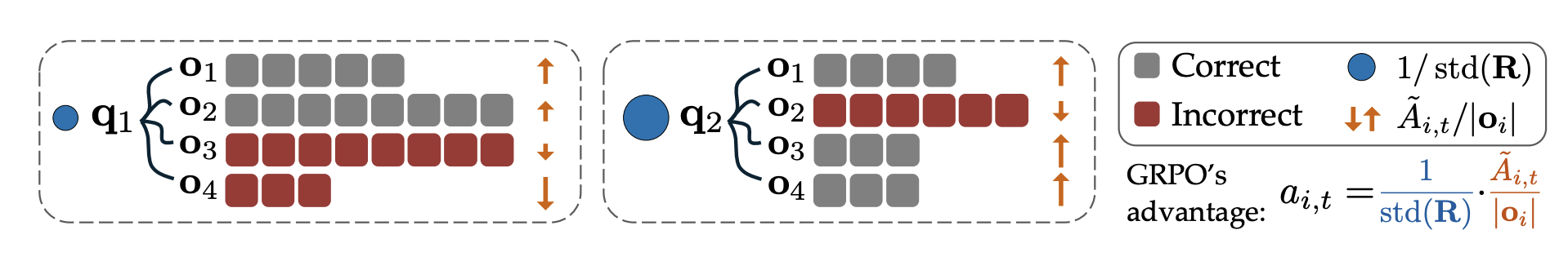
Bias 主要出在了 \(\sigma\) 上，我们接下来具体分析它带来的影响:

• 当某个 prompt 的 group 里 奖励方差很小（组内Reward全对或者全错）时，\(\frac{1}{\sigma}\) 会非常大 → 这个 prompt 对梯度更新的权重被放大。
• 当奖励方差大时，更新被缩小。

这就会导致，训练过程中，模型会更关注“极端题”（全对/全错），而不是“中等难度、最能学到东西的题”。

Question: 为什么，\(\mu\)（组内均值）不会带来Bias呢？

因为 \(\mu\) 只是一个平移，它不会改变梯度的权重，只会改变梯度的方向（让模型更关注相对更好的回答）。而 \(\sigma\) 是一个缩放，它会改变梯度的权重，从而引入Bias。

3.4.2 Length Normalization Bias

在 Equation 1 中，有一个 按回答长度归一化 的项 \(\frac{1}{|o_i|}\)，也就是把每条回答的 token-loss 平均化。

这会带来response-level length bias：当把一条回答的梯度按长度平均时，会改变“同样一条回答”在优化中的有效权重。（很抽象对不对，我们来看两个具体情况）

1. 优势为正（答对/更好，\(\hat{A} > 0\)） 在这种情况下，更新方向是“提高这条回答概率”，但除以回答长度 \(|o_i|\)，这意味着越短的回答，单位长度的梯度越大， 每个 token 的贡献更大。于是，模型学到：正确答案要尽量短（因为更“划算”）。

2. 优势为负（答错/更差，\(\hat{A} < 0\)） 在这种情况下，更新方向是“降低这条回答概率”（惩罚），但除以回答长度 \(|o_i|\)，这意味着越长的回答，惩罚被摊薄，每个 token 的负更新更小。于是，模型学到：错误答案反而更愿意写长（因为“受罚更轻”）。

这就是为什么有时候CoT越来越长，但是Reward还是不升反降的现象——模型学会了通过输出更长的回答来“规避惩罚”，而不是通过提高回答质量来获得更高的奖励。

Figure 4: 该张图展示了 DeepSeek-R1-Zero 在训练过程中，模型平均每条回答长度随训练步数的变化。横轴是训练步数（Steps），纵轴是平均每条 response 的长度（token 数）。可以看到，随着训练推进，模型输出长度呈持续上升趋势：从训练初期的几百到上千 token，逐步增长到后期的一万甚至接近两万 token，同时波动幅度也明显扩大。这一现象直观反映了 R1-Zero 在仅使用可验证奖励进行强化学习时，模型倾向于生成越来越长的推理链（CoT），体现出典型的“长度膨胀”行为，而不一定对应更高的实际解题效率。

接下来，我们来看 Dr.GRPO(Liu et al. 2025) 是如何解决这两个问题的。

3.5 Dr.GRPO

Dr.GRPO 是 GRPO 的一个变体，解决了上面提到的两个问题：

• 去掉 \(\frac{1}{\sigma}\)，避免 biased gradient
• 去掉按回答长度归一化，避免长度偏置

我们来看看改动之后的目标函数:

\[ \mathcal{J}_{\text{Dr.GRPO}}(\pi_\theta) = \frac{1}{G}\sum_{i=1}^{G} \sum_{t = 1}^{|o_i|} \Bigg\{ \min \Big[ \rho(o_{i,t}) \hat{A}_{i, t}, \text{clip}\Big( \rho(o_{i,t}), 1 - \epsilon_{\text{clip}}, 1 + \epsilon_{\text{clip}} \Big) \hat{A}_{i, t} \Big] \Bigg\} \tag{9}\]

其中，Advantage 变成：

\[ \hat{A}_{i, t} = r_i - \mu \quad \text{where} \quad \mu = \frac{1}{G}\sum_{j=1}^{G} r_j \tag{10}\]

也就是只用组内均值当 baseline，不做方差归一化。

另一个改动是去掉了按回答长度归一化，也就是不再除以 \(|o_i|\)， 直接对所有 token 的 policy-gradient loss 求和。 不过在实现中，会除以一个MAX_TOKENS（最大token数）来稳定训练，但这个是个常数，不会引入长度偏置。

我们来看看代码

def compute_loss_grpo(
    log_probs: torch.Tensor,      # (B, G, T) log probs under current policy
    old_log_probs: torch.Tensor,  # (B, G, T) log probs under old policy (detached)
    response_mask: torch.Tensor,  # (B, G, T) mask for valid response tokens
    advantage: torch.Tensor,    # (B, G) advantage per response
    clip_range: float = 0.2,
    max_tokens: int = 1024,
):
    B, G, T = log_probs.size()

    important_ratio = torch.exp(log_probs - old_log_probs)  # (B, G, T)

    # Broadcast advantage to token level
    advantage_tok = advantage.unsqueeze(-1).expand_as(important_ratio)  # (B, G, T)

    unclipped = important_ratio * advantage_tok
    clipped = torch.clamp(important_ratio, 1 - clip_range, 1 + clip_range) * advantage_tok

    pg_loss_tok = -torch.min(unclipped, clipped)  # (B, G, T)

    # Length normalization (GRPO does this)
    pg_loss_tok = pg_loss_tok * response_mask  # mask out non-response tokens 
    pg_loss_seq = pg_loss_tok.sum(dim=-1) / max_tokens  # (B, G) 

    # Final loss: mean over batch and group
    loss = pg_loss_seq.sum()
    loss = loss / (B * G)
    # loss = pg_loss_seq.mean()  # alternative: mean over all tokens

    return loss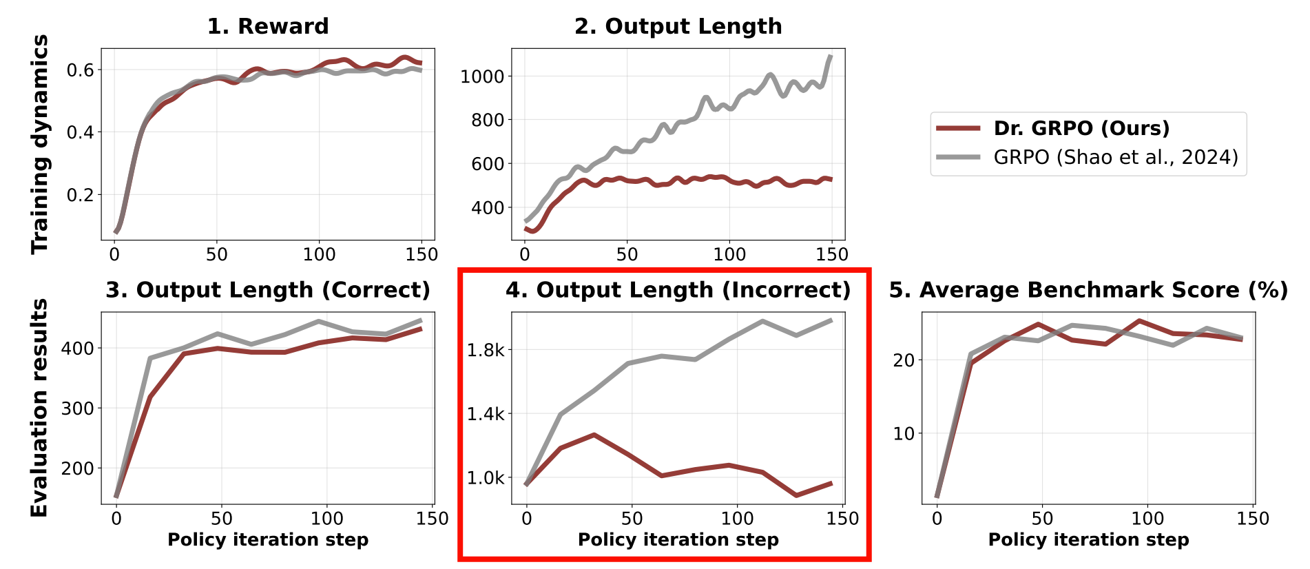

Figure 5: 主要看图中红色部分，Dr.GRPO在错误回答时，不再按长度归一化，这样长回答不会被“惩罚更轻”，从而避免了模型学会写长错误回答的现象。

4 Case Studies

在了解了GRPO算法后，我们来看看它是如何在实际例子中应用的，包括 DeepSeek-R1、Kimi 1.5 和 Qwen 3 等模型。

4.1 DeepSeek-R1

DeepSeek-R1 在2025年春节期间发布（还记得当时铺天盖地全是DeepSeek的新闻，过年都被卷到），它是第一个用 GRPO 做数学推理强化学习的模型。接下来我们来一下DeepSeek R1 (DeepSeek-AI et al. 2025)是如何训练的。

WARNING: 关于DeepSeek-R1 Paper与课堂上的不同

DeepSeek R1 在最近（2026年1月）重新Release了它们新的训练细节论文，该笔记基于最新论文内容进行整理。而课程中是基于最初的技术报告进行讲解，二者在细节上可能存在差异。

首先，我看一下DeepSeek R1的整体pipeline：

Figure 6

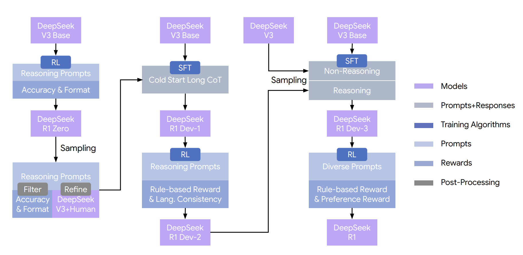
DeepSeek R1 并不是一次性通过强化学习训练出来的模型，而是一条多阶段、逐步增强推理能力的训练流水线。

4.1.1 From DeepSeek-V3 to DeepSeek-R1-Zero

从 DeepSeek V3 Base 出发，研究者首先进行了几乎“纯 RL”的实验（R1-zero）：仅在推理类 prompt 上，用 accuracy 与 format 这类可验证的 outcome-level 奖励进行强化学习，验证一个关键假设——在没有 process supervision 的情况下，RL 是否足以激活模型的推理能力。

Specifically, we apply the RL technique on the DeepSeek-V3 base to train DeepSeek-R1-Zero. During training, we design a straightforward template, to require DeepSeek-R1-Zero to first produce a reasoning process, followed by the final answer. We intentionally limit our constraints to this structural format, avoiding any content-specific biases to ensure that we can accurately observe the model’s natural progression during the RL process. DeepSeek-R1: Incentivizing Reasoning Capability in LLMs via Reinforcement Learning, p.4

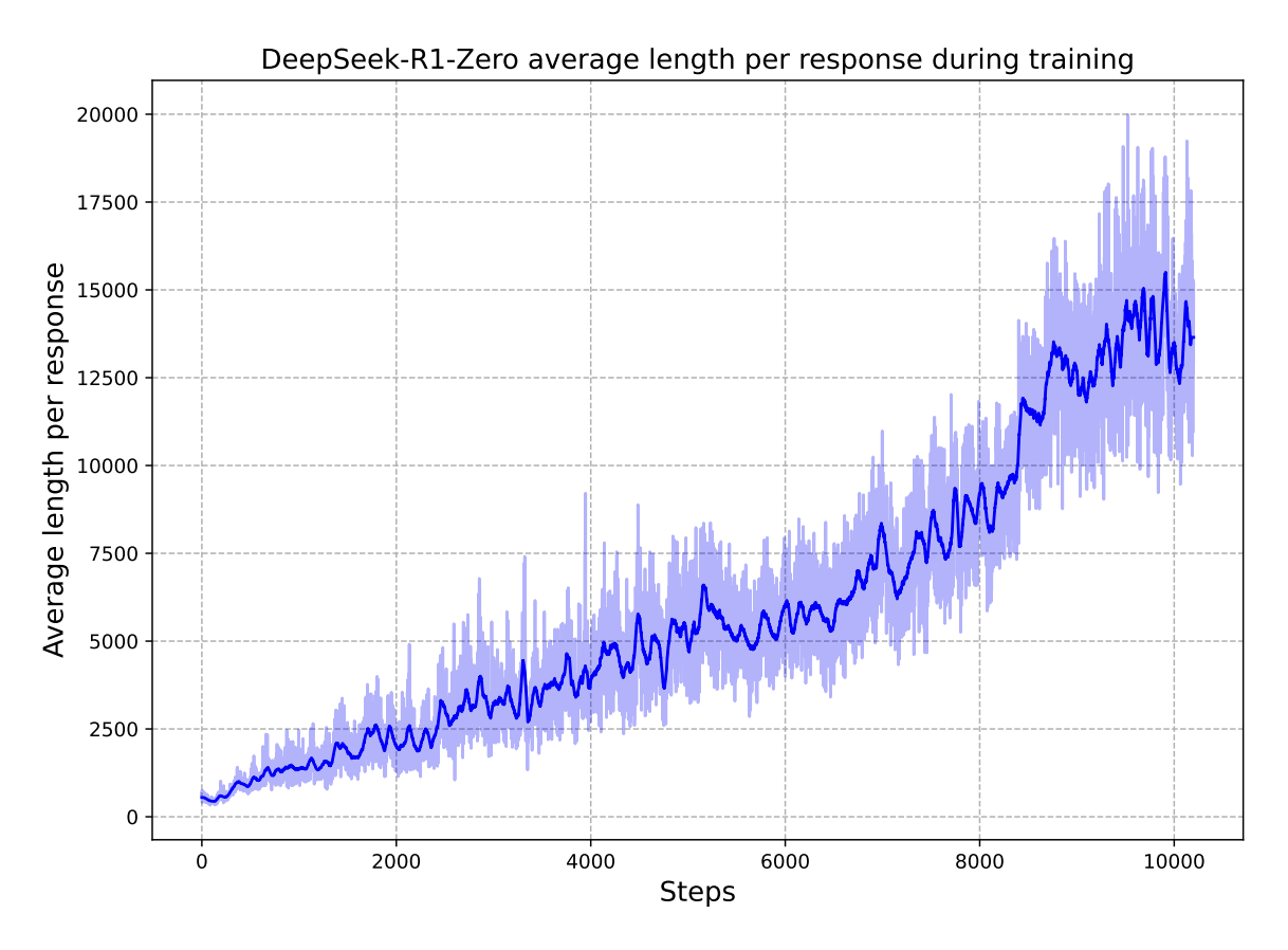
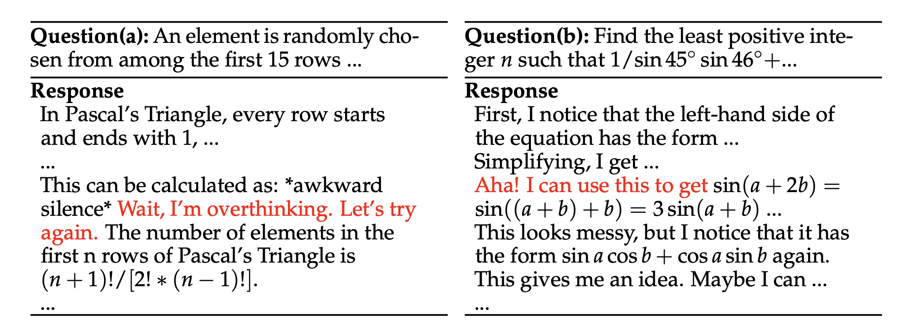
结果表明推理能力确实可以被激发，同时发现了 “aha moment” 现象：模型在训练过程中会突然开始生成更长、更复杂的 CoT，伴随推理正确率的显著提升。

Notably, during training, DeepSeek-R1-Zero exhibits an “aha moment” characterized by a sudden increase in the use of the word “wait” during reflections DeepSeek-R1: Incentivizing Reasoning Capability in LLMs via Reinforcement Learning, p.5

DeeoSeek R1-zero 的成功验证了 RLVR 思路的可行性：即使没有 process-level supervision，仅凭 outcome-level 的可验证奖励，RL 也能激发 LLM 的推理能力。

The self-evolution of DeepSeek-R1-Zero underscores the power and beauty of RL: rather than explicitly teaching the model how to solve a problem, we simply provide it with the right incentives, and it autonomously develops advanced problem-solving strategies. DeepSeek-R1: Incentivizing Reasoning Capability in LLMs via Reinforcement Learning, p.5

不过课程中提到，CoT 变长、“aha/backtracking”等现象；可能是来自目标/实现细节的偏置，不一定是“学会更深思考”的必然， “aha”这类文本也可能在底座模型上偶发出现，不必过度神化“涌现”。

Figure 7: shows two examples to demonstrate that the DeepSeek-V3-Base model already exhibits the so-called “aha moment” even before the RL-tuning (Image Source (Liu et al. 2025))

在这个阶段，DeepSeek R1-zero 的训练采用了 GRPO Algorithm 1 算法，并设计了专门的奖励函数：

• Outcome-level 奖励：主要包括 accuracy 奖励（答案正确与否）和 format 奖励（输出格式是否符合要求）

4.1.2 From DeepSeek-R1-Zero to DeepSeek-R1

DeepSeek-R1-zero 很好，但是它存在几个问题：

Although DeepSeek-R1-Zero exhibits strong reasoning capabilities, it faces several issues. DeepSeek-R1-Zero struggles with challenges like poor readability, and language mixing, as DeepSeek-V3-Base is trained on multiple languages, especially English and Chinese. DeepSeek-R1: Incentivizing Reasoning Capability in LLMs via Reinforcement Learning, p.6

因此，在R1-zero的基础上，DeepSeek团队设计了 DeepSeek-R1 的训练方案，来提升模型的表达质量与行为 稳定性。具体来说：

• SFT 冷启动：利用 R1-zero 采样得到的大量推理轨迹，经过过滤与人工/模型精修后，对 V3 Base 进行 Cold-start Long CoT 的 SFT，得到 R1 Dev 系列模型；
• 多轮 GRPO 式 RL：随后再通过多轮 GRPO 式 RL，引入语言一致性奖励、偏好奖励以及更丰富的任务分布，逐步把模型从“只会解题”推向“推理强、表达稳定、行为可控”的产品级模型。

In the initial stage, we collect thousands of cold-start data that exhibits a conversational, human-aligned thinking process. RL training is then applied to improve the model performance with the conversational thinking process and language consistency. Subsequently, we apply rejection sampling and SFT once more. This stage incorporates both reasoning and nonreasoning datasets into the SFT process, enabling the model to not only excel in reasoning tasks but also demonstrate advanced writing capabilities. To further align the model with human preferences, we implement a secondary RL stage designed to enhance the model’s helpfulness and harmlessness while simultaneously refining its reasoning capabilities. DeepSeek-R1: Incentivizing Reasoning Capability in LLMs via Reinforcement Learning, p.6

同时，DeepSeek R1 也在奖励设计上做了改进：

• 多维奖励设计：不仅包含可验证的 outcome-level 奖励（accuracy、format），还引入了Language consistency reward、Preference / non-verifiable rewards（通过对比学习训练的偏好模型）等，更全面地衡量模型输出质量；
• 奖励混合与调优：通过对不同奖励进行加权混合与调优，确保模型在提升推理能力的同时，也能兼顾表达质量与行为稳定性。
• 持续的奖励模型训练：在 RL 训练过程中，持续更新奖励模型，以适应模型能力的提升与任务分布的变化。

4.1.3 DeepSeek Distillation

在 DeepSeek R1 训练完成后，研究者还进行了蒸馏（distillation），以提升模型的推理效率与实用性.

To enable broader access to powerful AI at a lower energy cost, we have distilled several smaller models and made them publicly available. DeepSeek-R1: Incentivizing Reasoning Capability in LLMs via Reinforcement Learning, p.2

具体的方法就是：用 R1 作为 teacher 模型，生成大量高质量的推理样本，然后对更小的 student 模型进行 SFT 蒸馏训练。

For distilled models, we apply only SFT and do not include an RL stage, even though incorporating RL could substantially boost model performance. DeepSeek-R1: Incentivizing Reasoning Capability in LLMs via Reinforcement Learning, p.60

4.2 Kimi 1.5

和 DeepSeek R1 更像“配方驱动（SFT→RL→再对齐）”不同，课程把 Kimi 1.5 的经验总结成一句话：data is king。Kimi 的核心不是提出全新 RL 算法，而是把“可验证奖励推理 RL”变成一条更工程化的数据管线：先对任务做跨领域分类与分布平衡，避免模型只在单一类型题上变强；同时主动剔除容易通过随机猜测获得奖励的题型（例如选择题、判断题），优先保留短答案、可被规则/判定器高精度验证的任务，以减少 reward hacking 的空间。

最关键的一步是 best-of-n 难度筛选：用当前还不够强的 SFT 模型对每道题采样多次（课上举例类似 best-of-8），然后只保留“采样多次仍然失败”的题（fail best-of-n）。直觉上，这相当于把训练数据限制在“当前模型确实不会，但又可能学会”的可学区间，显式做出一种 curriculum 的雏形：太容易的题学不到东西，太难的题只会产生大量 0 reward；而经过筛选的题更可能提供稳定的学习信号。课程的 takeaway 是：在 RLVR 场景里，数据难度控制往往比算法 tweak 更决定训练效率和最终行为。

4.3 Qwen3

课程在讲 Qwen3 时，强调它的亮点不只是“也用了 RLVR/GRPO”，而是把推理模型在真实使用场景里的一个核心矛盾摆到台面上：推理越强，往往越贵（更长的 CoT、更高的 test-time compute）。因此 Qwen3 的思路更像是把“推理能力”和“推理成本”一起纳入训练目标：一方面沿用 “SFT（长 CoT 冷启动）→ 可验证奖励 RL（提升推理正确性）→ 再做通用对齐” 的主线；另一方面通过训练与数据/奖励设计，让模型学会在不同问题上自适应地选择推理强度——该认真推时能推得深，不需要推理时也能走更短、更便宜的路径。

从课程视角看，Qwen3 体现了一种很实用的产品化取向：推理模型最终要在“正确率”和“成本/延迟”之间做权衡，单纯追求 CoT 变长并不等价于更好。与 DeepSeek R1 更强调“用 RL 激活推理”以及 Kimi 更强调“用数据筛选做 curriculum”相比，Qwen3 更像是在探索：如何把“计算预算可控”变成模型行为的一部分，从而避免 RL 训练把 CoT 拉爆、成本失控的副作用。

5 GRPO Implementation

接下来我们通过一个简单的例子，来具体看看GRPO的算法。这个例子是来自 Lecture17group baseline / 标准化优势 / clip ratio 这些 GRPO/PPO 家族的核心机制, 我们会根据 Algorithm 1 中的伪代码，一步步实现 GRPO。

5.1 Data & Goal

任务：排序（Sorting）

• Prompt：长度为 LLL 的整数序列，例如 [3, 1, 2, 0]
• Response：模型输出同样长度 LLL 的序列，希望是排序后的结果 [0, 1, 2, 3]
• group 结构（GRPO 的关键）：对同一个 prompt，采样 \(k\) 条 response \(\{a^{(1)}, a^{(2)}, \dots, a^{(K)}\}\) 形成一组，用于计算组内 baseline（均值/标准差）。

def gen_prompts(batch_size: int, seq_len: int, vocab_size: int, device) -> torch.Tensor:
    return torch.randint(low=0, high=vocab_size, size=(batch_size, seq_len), device=device)


def sorted_ground_truth(prompt: torch.Tensor) -> torch.Tensor:
    return torch.sort(prompt, dim=-1).values

5.2 Reward

首先我们需要定义 reward 函数。Lecture 里强调：如果 reward 只给 0/1（完全正确/错误），会导致稀疏奖励，训练很容易卡住。因此这里使用 partial credit来让学习更平滑。

5.2.1 Reward v2：Inclusion + Adjacent Sorted Pairs（课堂采用的更细奖励）

给定 prompt \(x\) 和 response \(y\)：

1. Inclusion reward：prompt 里的 token 在 response 里出现就给分（按计数，多重集）

\[ \text{Inclusion reward:} \quad R_{\text{inc}}(x,y)=\sum_{t} \min(\text{count}_x(t), \text{count}_y(t)) \tag{11}\]

2. Adjacent sorted pairs：统计 response 中相邻对满足非降序的个数

\[ \text{Adjacent sorted pairs:} \quad R_{\text{adj}}(y)=\sum_{i=1}^{L-1}\mathbb{I}[y_i \le y_{i+1}] \tag{12}\]

总 reward：

\[ \text{Total reward:} \quad R(x,y)=R_{\text{inc}}(x,y)+R_{\text{adj}}(y) \tag{13}\]

课堂也提到：这种 reward 可能存在“漏洞”（reward hack），因此 reward 设计本身就是 RL 的难点之一。

def sort_distance_reward(prompt: list[int], response: list[int]) -> float:
    assert len(prompt) == len(response)
    ground_truth = sorted(prompt)
    return sum(1 for x, y in zip(response, ground_truth) if x == y)


def sort_inclusion_ordering_reward(prompt: list[int], response: list[int]) -> float:
    """
    Return how close response is to ground_truth = sorted(prompt).
    """
    assert len(prompt) == len(response)
    # Give one point for each token in the prompt that shows up in the response
    inclusion_reward = sum(1 for x in prompt if x in response)  # @inspect inclusion_reward
    # Give one point for each adjacent pair in response that's sorted
    ordering_reward = sum(1 for x, y in zip(response, response[1:]) if x <= y)  # @inspect ordering_reward
    return inclusion_reward + ordering_reward

5.3 Model

对于这个任务，我们就定一个简单的模型：

class ToySortPolicy(nn.Module):
    def __init__(self, vocab_size: int, embedding_dim: int, prompt_length: int, response_length: int):
        super().__init__()

        self.embedding_dim = embedding_dim
        self.emb = nn.Embedding(vocab_size, embedding_dim)
        self.enc = nn.Parameter(
            torch.randn(prompt_length, embedding_dim, embedding_dim) / math.sqrt(embedding_dim)
        )
        self.dec = nn.Parameter(
            torch.randn(response_length, embedding_dim, embedding_dim) / math.sqrt(embedding_dim)
        )
        self.out = nn.Linear(embedding_dim, vocab_size)

    def forward(self, prompt):
        x = self.emb(prompt)  # (B,L,d1)
        h = torch.einsum("bld,ldm->bm", x, self.enc)  # (B,d2)
        z = torch.einsum("bm,lmd->bld", h, self.dec)  # (B,L,d1)
        return self.out(z)  # (B,L,V)

5.4 Algorithm

def grpo(cfg: GRPOCfg = GRPOCfg()):
    dev = get_device()
    set_seed(cfg.seed)

    policy = ToySortPolicy(cfg.V, cfg.L, cfg.L, cfg.L).to(dev)
    opt = torch.optim.Adam(policy.parameters(), lr=cfg.lr)

    reward_fn = REWARD_FN_MAP[cfg.reward_fn]

    # reference model (slow-moving anchor for KL)
    ref = ToySortPolicy(cfg.V, cfg.L, cfg.L, cfg.L).to(dev)
    ref.load_state_dict(policy.state_dict())
    ref.eval()

    for it in range(cfg.outer_iters):
        # update reference model slowly
        if cfg.use_kl and it > 0 and (it % cfg.ref_update_every == 0):
            ref.load_state_dict(policy.state_dict())
            ref.eval()

        # ---------- OUTER: rollout + rewards + deltas + freeze old/ref logps
        prompt = gen_prompts(cfg.B, cfg.L, cfg.V, dev)  # (B,L)

        with torch.no_grad():
            responses = sample_responses(policy, prompt, cfg.K, cfg.temperature)  # (B,K,L)
            rewards = compute_reward(prompt, responses, reward_fn)  # (B,K)
            deltas = compute_deltas(rewards, cfg.delta_mode)  # (B,K)

            # IMPORTANT: freeze old logps (detach)
            old_logp_token = compute_log_probs(prompt, responses, policy).detach()  # (B,K,L)

            # freeze ref logps for KL (detach)
            ref_logp_token = compute_log_probs(prompt, responses, ref).detach() if cfg.use_kl else None

        # ---------- INNER: multiple gradient steps on same samples
        for _ in range(cfg.inner_steps):
            opt.zero_grad(set_to_none=True)

            logp_token = compute_log_probs(prompt, responses, policy)  # (B,K,L)

            loss = compute_loss(
                log_probs=logp_token,
                old_log_probs=old_logp_token,
                deltas=deltas,
                mode=cfg.loss_mode,
            )

            if cfg.use_kl:
                loss = loss + cfg.kl_beta * compute_kl_penalty(logp_token, ref_logp_token)

            loss.backward()
            opt.step()

        if (it % cfg.print_every) == 0 or it == cfg.outer_iters - 1:
            with torch.no_grad():
                print(
                    f"iter {it:04d} | "
                    f"reward mean {rewards.mean().item():.3f} "
                    f"(min {rewards.min().item():.1f}, max {rewards.max().item():.1f}) | "
                    f"loss {loss.item():.4f}"
                )

    return policy

5.5 Training

@dataclass
class GRPOCfg:
    V: int = 10  # vocab size (token values 0..V-1)
    L: int = 4  # sequence length
    B: int = 128  # batch prompts per outer iter
    K: int = 8  # responses per prompt (group size)
    outer_iters: int = 200
    inner_steps: int = 4

    lr: float = 2e-2
    temperature: float = 1.0

    delta_mode: Literal["raw", "centered_rewards", "normalized_rewards", "max_rewards"] = "centered_rewards"
    loss_mode: Literal["naive", "unclipped", "clipped"] = "clipped"
    clip_eps: float = 0.2

    use_kl: bool = True
    kl_beta: float = 0.02
    ref_update_every: int = 30

    seed: int = 0
    print_every: int = 20

    reward_fn: Literal["distance", "inclusion_ordering"] = "inclusion_ordering"

5.6 Results

iter 0000 | reward mean 3.070 (min 0.0, max 7.0) | loss 0.0138
iter 0020 | reward mean 3.250 (min 0.0, max 6.0) | loss 0.0034
iter 0040 | reward mean 3.396 (min 0.0, max 7.0) | loss 0.0008
iter 0060 | reward mean 3.625 (min 0.0, max 7.0) | loss 0.0016
iter 0080 | reward mean 3.813 (min 1.0, max 7.0) | loss 0.0059
iter 0100 | reward mean 4.071 (min 1.0, max 7.0) | loss 0.0043
iter 0120 | reward mean 4.278 (min 1.0, max 7.0) | loss 0.0030
iter 0140 | reward mean 4.497 (min 1.0, max 7.0) | loss 0.0058
iter 0160 | reward mean 4.710 (min 1.0, max 7.0) | loss 0.0058
iter 0180 | reward mean 4.859 (min 2.0, max 7.0) | loss 0.0033
iter 0199 | reward mean 4.964 (min 2.0, max 7.0) | loss 0.0067


=== sample check ===
prompt: [4, 2, 4, 4] | pred: [0, 2, 4, 6] | gt: [2, 4, 4, 4] | sort reward: 1 | inclusion+ordering reward: 7
prompt: [6, 8, 1, 9] | pred: [8, 9, 1, 1] | gt: [1, 6, 8, 9] | sort reward: 0 | inclusion+ordering reward: 5
prompt: [4, 3, 8, 7] | pred: [0, 3, 6, 7] | gt: [3, 4, 7, 8] | sort reward: 0 | inclusion+ordering reward: 5
prompt: [6, 0, 5, 6] | pred: [0, 5, 7, 9] | gt: [0, 5, 6, 6] | sort reward: 2 | inclusion+ordering reward: 5
prompt: [3, 1, 4, 6] | pred: [1, 1, 4, 7] | gt: [1, 3, 4, 6] | sort reward: 2 | inclusion+ordering reward: 5
prompt: [2, 7, 8, 0] | pred: [3, 7, 7, 8] | gt: [0, 2, 7, 8] | sort reward: 2 | inclusion+ordering reward: 5
prompt: [7, 9, 1, 2] | pred: [9, 9, 1, 9] | gt: [1, 2, 7, 9] | sort reward: 1 | inclusion+ordering reward: 4
prompt: [3, 6, 0, 2] | pred: [1, 1, 3, 7] | gt: [0, 2, 3, 6] | sort reward: 1 | inclusion+ordering reward: 4

全部的代码可以在这个Notebook中看到

6 Summary

在这篇笔记中，我将 Lecture 16 与 Lecture 17 合并整理，围绕一个核心问题展开：为什么传统的 PPO 与 DPO 已不足以支撑推理型 LLM 的强化学习，以及 RLVR（Reinforcement Learning from Verified Rewards）如何成为新的突破口。我首先回顾了 PPO、DPO 在推理场景中的工程复杂度与数据形态局限，并由此引出 GRPO 这一代表性算法，系统梳理了其目标函数、基于 group 的相对 advantage 计算、clip ratio、KL 约束以及长度归一化等关键设计。在此基础上，我进一步分析了 GRPO 中两个重要但容易被忽略的偏置来源：一是由组内奖励标准差引入的 biased gradient，二是按回答长度归一化导致的 length bias，并结合 Dr.GRPO 展示了通过去除 1/与 length normalization 来缓解这些问题的思路。最后，我从课程视角总结了 DeepSeek-R1、Kimi 1.5 与 Qwen3 在 RLVR 实践中的不同取向，并通过一个排序任务的 toy 示例，完整实现了 GRPO 的数据生成、奖励设计、模型结构与训练流程，将算法从公式推导真正落到可运行的代码层面。 # Further 在完成了这三节课程之后，我们可以开始Assignment05的实现，在Assignment05中，我们会实现3中算法：

• SFT
• Expert Iteration
• GRPO

并且比较它们的不同，具体的代码实现可以参考GitHub， 以及对应的笔记。

7 In the End

最后，感谢你一路坚持到这里！创作不易，如果你觉得内容对你有帮助，欢迎请我喝杯咖啡/支付宝红包，支持我继续创作！你们的支持是我最大的动力！ :)

References

DeepSeek-AI, Daya Guo, Dejian Yang, Haowei Zhang, Junxiao Song, Peiyi Wang, Qihao Zhu, et al. 2025. “DeepSeek-R1: Incentivizing Reasoning Capability in LLMs via Reinforcement Learning.” Nature 645 (8081): 633–38. https://doi.org/10.1038/s41586-025-09422-z.

Liu, Zichen, Changyu Chen, Wenjun Li, Penghui Qi, Tianyu Pang, Chao Du, Wee Sun Lee, and Min Lin. 2025. “Understanding R1-Zero-Like Training: A Critical Perspective.” October 6, 2025. https://doi.org/10.48550/arXiv.2503.20783.

Shao, Zhihong, Peiyi Wang, Qihao Zhu, Runxin Xu, Junxiao Song, Xiao Bi, Haowei Zhang, et al. 2024. “DeepSeekMath: Pushing the Limits of Mathematical Reasoning in Open Language Models.” April 27, 2024. https://doi.org/10.48550/arXiv.2402.03300.